Completing Facades

Introduction

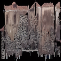
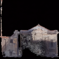
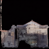
Venice is a unique city with both cultural and historical significance. Digital copies of cities allows us to preserve and understand them better. Photogrammetry is a technology that can be used to do this which uses images and scans to create models of real world objects and sites. However, due to the nature of the technology there are often holes, missing regions and noise in the data. This project aims to fill in holes in data from photogrammetry of facades in Venice by also using historical data over buildings in Venice. For this 2D images from photogrammetry of Venice is used. The dataset used includes completed and incomplete facades. To achieve this aim a method for generating artificial holes in facades was developed together with a dataset of facades with artificial holes and the binary mask for the created missing regions. A machine learning method for detecting the holes in the facades was developed. Additionally, two methods for alining footprints of Venice buildings was implemented in order to align a hand drawn map with the footprint of Venice. ...Finally, a neural network was trained on different ... For the filling of the holes GAN was used.

Motivation and description of the deliverables

Dataset with generated holes

This data set was created in order to train a model on detecting holes.

Model for identifying holes

This model was created in order to fill the missing regions of facades. Prevent noise, filling or reconstructing regions which we are not wanting to reconstruct.

Project Timeline & Milestones

For this project, GitHub served as the project management tool. It was used to organize tasks, track progress, and develop a project timeline. The first week of the project was spent setting up our environments, loading in the data for the project and exploring it. This work continued in the second week and we started to defining our pipeline and the fist step of the pipeline was to fill in the holes in the facades. To optimize our work we also started working on attaching the cadastre data to the facades and then preparing for the presentation. The project timeline was structured around specific milestones for after the midterm presentation in order to complete the pipeline for filling in the facades. Figure 2.1 illustrates the progress of tasks before the midterm presentations and the milestones after the midterm presentation.

Figure 2.1: Timeline over project from midterm presentation

Three major milestones were defined for the remaining work together with writing and preparing for the final presentation.

The first milestone:

• Completing the detection of holes in facades
• Completing attaching cadastre data to the building footprints
• Literature review of hole filling methods

The second milestone:

• Group facades by attributes
• Start exploring and developing hole filling methods

The final milestone:

• Development and refinement of the model to fill in the detected holes in the facades
• Writing and preparing for the presentation

The table below shows a weekly project overview.

Project timeline

Week	Task	Status
07.10 - 13.10	Set up python environments, explore dataset, structure work on Github	Done
14.10 - 20.10	Document and explore dataset and start defining pipeline	Done
21.10 - 27.10	Autumn vacation
28.10 - 03.11	Work on detecting holes, attaching cadastre data to footprints of Venice
04.11 - 10.11	Work on detecting holes, attaching cadastre data to footprints of Venice. Prepare for the presentation ||
11.11 - 17.11	Midterm presentation on 14.11. Finish attaching cadastre data to footprints of Venice and hole detection method. ||
18.11 - 24.11	Finish attaching cadastre data to footprints of Venice and hole detection method. Litterature review of hole filling method ||
25.11 - 01.12	Sort and group facades by different attributes, work on hole filling method, start writing.
02.12 - 08.12	Sort and group facades by different attributes, work on hole filling method, start writing
09.12 - 15.12	Finish writing wiki, Prepare presentation
16.12 - 22.12	Deliver GitHub + wiki on 18.12 Final presentation on 19.12

Methodology

In order to fill the holes in the images they first need to be detected.

Attaching historical data to facades data

In order to get historical data over the facades in Venice Cadastre 1808 was used. The data is a GeoDataFrame with polygons over the buildings in Venice and it contains historical information about the buildings such as ownership type. The polygons are from a hand drawn map of Venice and the buildings in Venice have also changed which has resulted in miss alignment of the buildings from the historical data with the current footprint of Venice. Thus, in order to attach the historical data to the facades a method for filtering out buildings and shifting the polygons has been developed.

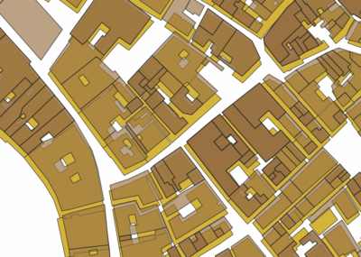
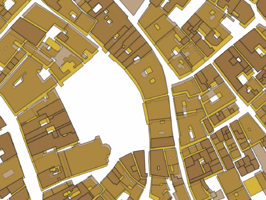
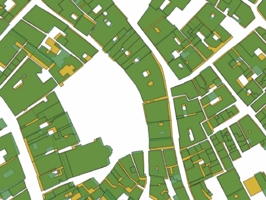
To align the datasets the current footprint of Venice the Edifici data was used mainly because of the difference in geometry between the cadastre buildings and the buildings of Venice today. Cadastre buildings are often smaller and simply attaching them to the closest facade would not provide good results because of the differences in geometry, to illustrate this and the miss alignment see figure 3.1, where cadastre buildings are shown in brown and Edifici buildings in yellow.

Figure 3.1: Edifici buildings are yellow and cadastre buildings are brown.

To better align the two maps, initial filtering of the data was done, since some Edifici buildings do not have any facade in the point cloud. These were filtered out to decrease the amount of data. Furthermore, there are duplicate entries of the same cadastre building in the dataset, this is not relevant when shifting the polygons thus these cases were also filtered out.

Two different metrics where used and evaluated for shifting the facades, percentage overlap and hausdorff distance. Percentage overlap between polygon A and B is defined as: Percentage overlap(A, B) = (|A ∩ B|) / A This was done for both Edifici and Cadastre polygons as there are cases where the Edifici polygon is smaller than the Cadastre polygon and vice versa. The Hausdorff distance is defined as the maximum distance between two polygons A and B. In this project, it was calculated by first joining all polygons overlapping an Edifici building and then computed using the hausdorff_distance method in GeoPandas.

The general approach for aligning and filtering the polygons can be outlined as follows:

1. Calculate metric

For every polygon in Edifici and Cadastre that overlap, calculate the metrics: percentage overlap and Hausdorff distance.

2. Filter buildings

Remove buildings that do not meet the specified criteria for percentage overlap or Hausdorff distance.

3. Identify easy cases

An easy case is a building that is well aligned in both maps. Easy cases were identified based on the metrics, either percentage overlap or Hausdorff distance.

4. Calculate offset between maps for easy cases

For every easy case, a vector between the centroids of the polygons in the two maps was calculated and stored.

5. Calculate the closest distance to an easy case and shift cadastre data

For every building in the cadastre dataset, the closest easy case was identified. The buildings in the Cadastre data were then all shifted by the vector in the closest easy case, multiplied by a learning rate smaller than 1.

6. Repeat until max iterations

For both methods, 25 iterations were used to shift the Cadastre polygons.

To compare the methods Jaccard index was used as the evaluation metric. The index distance is defined as: J(A, B) = 1 - (|A ∩ B|) / (|A ∪ B|) where:

• A and B are two building polygons.
• |A ∩ B| is the intersection area of A and B .
• |A ∪ B| is the size of their total area.

Model for filling holes

Based on our prior literature review, we found that many machine learning-based inpainting methods require manual definition of the regions to be filled. Fortunately, this step has already been completed. With the availability of masks for the holes, the process becomes significantly more straightforward. Our task is now more clearly defined as a specific inpainting problem.

At this stage, we aimed to test our images using various models, fine-tune those that meet our requirements, and compare their performance differences. The models we tried include Stable Diffusion, LaMa, and VAE. Our task requires the models to:

1. Automatically identify patterns in the image.

2. Successfully handle low-resolution images.

3. Effectively fill large missing regions in the image.

Results

Attaching historical data to facades data

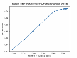
When shifting the facades for 25 iterations and using the metric percentage overlap the resulting average Jaccard index for the buildings is 0.548. The number of buildings kept after the final iteration is 5232 builings. See figure 4.1 for the results of the Jaccard index for each iteration.

• 

  Figure 4.1: Jaccard index when shifting the buildings for 25 iterations using metric percentage overlap.

• 

  Figure 4.2: Jaccard index when shifting the buildings for 25 iterations using metric Hausdorff distance.

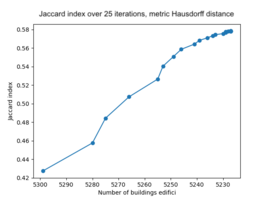
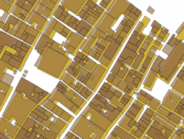
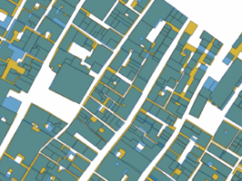
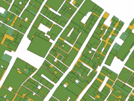
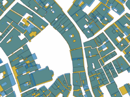
Using Hausdorff distance provides a higher resulting average Jaccard index of 0.578 after the final iteration and the number of buildings kept is 5227. See figure 4.2 for the results of the Jaccard index for each iteration. Filtering out buildings is done during the iterations and it is clear that this improves the overlap of the buildings. This is expected due to the difference in geometry of the Cadastre data and the Edifici data. Ideally, the performance when shifting the polygons would increase without buildings being removed, this would show that the shift improves the overlap of the buildings as well. This is less clear when looking at the performance of the Jaccard index. However, visually we can see the difference the shift makes, see figure 4.3 - 4.5.

• 
• 
• 
• 

  Figure 4.3: Original Edifici and Cadastre geometries.

• 

  Figure 4.4: Filtered Edifici and shifted Cadastre geometries using percentage overlap as metric.

• 

  Figure 4.5: Filtered Edifici and shifted Cadastre geometries using Hausdorff distance as metric.

However, as can be seen in the bottom figure 4.4 sometimes overlaps are created between the polygons after shifting, this is dicussed further in the discussion and limitations.

Based on our prior literature review, we found that many machine learning-based inpainting methods require manual definition of the regions to be filled. The great thing is that this step has already been completed. With the availability of masks for the holes, the process becomes significantly more straightforward. Our task is now more clearly defined as a specific inpainting problem.

Model for filling holes

Stable Diffusion

We began by using Stable Diffusion, a state-of-the-art text-to-image model that also supports inpainting. After conducting some initial tests, we present several examples of the generated images. As shown in Figure 4.3 and Figure 4.4, the pre-trained Stable Diffusion model struggles to fully capture the overall pattern of the image. The filled hole regions do not blend seamlessly with the existing areas; the generated regions and the original areas exhibit noticeably different styles. This issue may partly stem from the relatively low resolution of the images we need to inpaint.

• 

  Figure 4.3: Picture generated by using Stable Diffusion Inpainting.

• 

  Figure 4.4: Picture generated by using Stable Diffusion XL (SDXL) Inpainting.

Another issue lies with the prompts. We conducted some experiments to explore this further. As shown in Figure 4.5 and Figure 4.6, we tested the model with no prompts (`""`) and with prompts. While the generated images show differences between the two cases, they do not result in better outputs. Additionally, it remains unclear what prompts could be devised to enhance the model's performance for our specific task.

Also, there are certain special cases where Stable Diffusion fails to generate effective images, particularly when the hole regions are relatively large. In such instances, the generated images are often flagged as NSFW content and displayed entirely as black. See Figure 4.7.

• 

  Figure 4.5: Picture generated using Stable Diffusion Inpainting without prompt.

• 

  Figure 4.6: Picture generated using Stable Diffusion Inpainting with a prompt "venice facades, pixel, inpainting."

• 

  Figure 4.7: Generation failed due to "Potential NSFW content detected in one or more images. A black image was returned instead. Consider trying again with a different prompt and/or seed."

LaMa

After testing the Stable Diffusion model and encountering the aforementioned issues, we decided to shift our model strategy and identify a model more suitable for our task—automatically identifying patterns to fill missing regions without the need for prompts and demonstrating notable performance on low-resolution images. This led us to the LaMa model.

LaMa is a model designed for large-mask inpainting, introduced by Roman Suvorov et al. in 2021. It features a ResNet-inspired feed-forward inpainting network, incorporating fast Fourier convolution (FFC), a multi-component loss combining adversarial and high receptive field perceptual losses, and a training-time procedure for large mask generation. See Figure 4.8 for its structure.

Figure 4.8: Architecture of the LaMa model. Source: https://arxiv.org/pdf/2109.07161.pdf

LaMa offers several key advantages over Stable Diffusion, making it particularly well-suited for our inpainting tasks:

1. LaMa is lightweight and runs inference quickly, even on CPUs, whereas Stable Diffusion is computationally heavy and requires powerful GPUs.

2. Stable Diffusion relies on prompts, which can make its performance inconsistent and less predictable for our specific needs. While LaMa is deterministic and consistently produces the same output for the same input.

3. LaMa excels at completing repetitive or structured patterns. Stable Diffusion focuses on generating creative, diverse outputs rather than maintaining structured consistency.

Also, from our previous experiments, even though Stable Diffusion has more powerful capabilities, the low resolution of our images provides limited information for the model to learn from. As a result, Stable Diffusion fails to capture the patterns we need. This suggests that Stable Diffusion may not be well-suited for low-resolution images.

There are two versions of LaMa we can work with: one is the original model, and the other includes feature refinement proposed in https://arxiv.org/abs/2206.13644. We first conducted tests using both the original model and the feature-refinement-enhanced version to evaluate whether our images would perform better with the additional refinement.

Quality assessment and discussion of limitations

To assess the quality of the shift of the building the Jaccard Index was used. Furthermore, after shifting the buildings the results where analysed visually using QGIS. Additionally, after shifting overlaps between buildings are created and the number of overlaps were also calculated. Different methods for decreasing the number of overlapping buildings was tried such as decreasing the shift rate. Other approaches could be to only shift buildings within a certain radius or area? Or prevent shifts causing overlaps. However, doing this might also cause some buildings to never shift. Another way could be to identify more easy cases by decreasing the hausdorff distance or percentage overlap. Another metric such as average Hausdorff distance could also be used.

References

- ↑ R. A. Tabib, D. Hegde, T. Anvekar and U. Mudenagudi, "DeFi: Detection and Filling of Holes in Point Clouds Towards Restoration of Digitized Cultural Heritage Models," 2023 IEEE/CVF International Conference on Computer Vision Workshops (ICCVW), Paris, France, 2023, pp. 1595-1604, doi: 10.1109/ICCVW60793.2023.00175. keywords: {Point cloud compression;Geometry;Solid modeling;Three-dimensional displays;Pipelines;Data acquisition;Filling}
- ↑ Shapely: Hausdorff Distance, Shapely Documentation, access date: 2024-12-08, accessed: https://shapely.readthedocs.io/en/stable/manual.html#object.hausdorff_distance