Rolandi Librettos

The Rolandi Librettos can be considered as a collection of many unstructured documents, where each document describes an opera performance. Each document contains structured entity information about place, time and people (e.g.: composer, actors) who were involved in this opera. In our project we want to extract as much entity information about the operas as possible. This includes information as the title of the opera, when and in which city it was performed, who was the composer, etc. By extracting the entity information and linking it to internal and external entities, it is possible to construct one comprehensive data set which describes the Rolandi Collection. The linking of information to external entities, allows us to connect our data set to the real world. This for example includes linking every city name to a real place and assigning geographical coordinates (longitude and latitude) to it. Constructing links in the data set as such, allows us for example to trace popular operas which were played several times in different places or famous directors which directed many operas in different places. In a last step we construct one comprehensive end-product which represents the Rolandi Collection as a whole. Thus we want to visualize the distribution of operas Librettos in space and time and potentially construct indications of linking.

Example of libretto's coperta: Ama più chi men si crede

Example of libretto's coperta: Zenocrate a' Macedoni

Introduction

The Fondo Ulderico Rolandi is one of the greatest collections of librettos (text booklet of an opera) in the world. This collection of librettos which is in the possession of the Fondazione Cini consists of around 32’000 thousand librettos, spanning a time period from the 16th to the 20th century. This collection is being digitized and made accessible to the public in the online archives of the Fondazione Cini, where currently 1'110 librettos are available.

Motivation

This project is motivated by two main goals. Firstly, we would like to enrich the already existing metadata of the Cini Foundation on the Rolandi Librettos. The website already provides information about the title, the creator, and the year of representation of the libretto. This allows a user to query the libretto given a title, author, or by year and to quickly retrieve the former information. With our project, we would like to extract more entities in order to more accurately and extensively index and query the libretti. The entities we will extract are the title (a shorter version of the existing title metadatum, explained in section Title), city/place of representation, performance location (i.e. theater name, church, or other), the occasion (whether it was played at a Carnival or city fair), the genre of the opera and the composer or director of the play. Together with providing valuable indexing means, these features would allow users to carry out more extensive analyses on the corpus. For instance, it would allow to plot the distributions of the libretti in space, to extract the most flourishing theaters of the time, the most prolific composers. The creation of good, atomic, metadata would allow discerning which operas were played in more than one place, how the representation moved in space and time, which operas were put to music by the same composers, and much more.

Secondly, we would like to provide a comprehensive framework to visualize the extracted entities. This would allow the data to be easily understandable and interpretable. Specifically, the framework would allow to quickly identify time and place of representation of an opera, see what operas were played in the same period and location. It would allow zooming into the city and locating the theaters that were most prominent in the period, linking visually operas with the same title or composer, clicking on external links to Wikipedia pages and the original Cini archive.

In sum, the project is motivated by the will to extract and present information about this collection in a broad and accessible manner.

Realisation

We extracted the above entities, linked them to external and internal sources, visualized them, and served them on a website. Specifically, we created an environment to extract the appropriate entities from the IIIF manifests of the Cini Foundation. This environment can, in the future, be applied to the newly digitized libretti and extract the metadata mentioned above.

We applied our pipeline to 1100 already available libretti and extracted historically and culturally useful data. Some facts about the extracted data are reported in the tables below. From the tables, we could see that, unsurprisingly, the libretti come predominantly from Venice, followed by Rome. It is interesting to see that Reggio Emilia, a rather small town compared to the latter, was quite central when it came to opera representations. All the most frequent theaters extracted are in Venice, where the famous Teatro La Fenice already stands out as most prolific. Furthermore, selecting the most represented opera titles and composers we get an idea of what plays were most famous and which composers were the most requested.

Most common City Nr. Cities Number of Librettos 1 Venice 411 2 Rome 98 3 Reggio nell'Emilia 37 4 Bologna 29 5 Florence 26

Most common Theaters Nr. Theater City Number of Librettos 1 Teatro La Fenice Venice 92 2 Teatro di Sant'Angelo Venice 53 3 Teatro Giustiniani Venice 30 4 Teatro di S. Benedetto Venice 28 5 Teatro Vendramino Venice 21

Most Common Libretto Title Nr. Cities Number of Librettos 1 La vera costanza 7 2 Il geloso in cimento 7 3 Antigona 7 4 Artaserse 7 5 La moglie capricciosa 6

Most Common Composer Nr. Cities Number of Librettos 1 Giuseppe Foppa 14 2 Giovanni Bertati 13 3 Aurelio Aureli 9 4 Saverio Mercadante 8 5 Pietro Metastasio 6

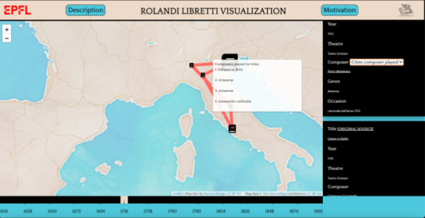
In order to further interpret the data and serve it in a comprehensive way, we created an interactive visualization and served it on a website. From the visualization, we could see which cities and theaters were most popular in which period, in which cities, and for what operas the same composer played, and how the same operas evolved in time and space. It also allowed us to quickly follow the external links to MediaWiki and read the dedicated pages of the composers and opera titles.

Methodology

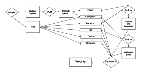
Our data processing pipeline consists conceptually of four steps: 1) Data collection 2) Data extraction 3) Data linking 4) Visualization. In practice, as the data extraction of different entities runs independently, those steps can run either in parallel or sequentially. Furthermore, the data source, which is in our case either the coperta or an extensive title for the libretto, from which we try to extract a given entity, also strongly influences the chosen methodology. Following, we will describe our data processing pipeline given those different circumstances and goals.

Data Collection

First, we use a scraper to obtain the metadata and the images for each libretto from the online librettos archive of the Cini Foundation. In the IIIF framework, every object or manifest, in our case librettos, is one .json document, which stores metadata and a link to a digitized version of the libretto. With the python libraries BeautifulSoup and request we could download those manifests and save them locally. Those manifests contained already entity information such as publishing year and a long extensive title description, which was extracted for each libretto.

Data Extraction

After obtaining the year, an extensive title description, and a link to the digitization, we were able to extract further entity information for each libretto from two main sources: The title description and the coperta's of the librettos.

Our pipeline from input data to visualization

Data Extraction from Copertas

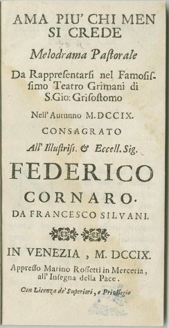
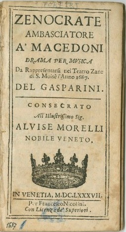
The coperta of a libretto corresponds to the book cover, which contains various information about the content and circumstances. A crucial feature for us was that only the coperte contained information about where the librettos were printed and distributed, which was only rarely included in the title information. Furthermore, the coperte sometimes also mentioned the names of the composers. To localize the librettos we, therefore, had to extract the city information from the coperte.
First, we downloaded the coperte from the Cini online archives. The coperte are specially tagged in the IIIF manifests, thus they could be downloaded separately.
Subsequently, we made the coperte machine-readable with an optical character recognition (OCR) algorithm. For this task we chose Tesseract, which has the advantages of being easily usable as python plugin and furthermore not having any rate limit or costs associated. This was advantageous, because we often reran our code or experimented also OCRing additional pages, therefore a rate limit would have been cumbersome. On the other hand, the OCR quality of Tesseract is very low, and because of lacking OCR quality, we were not able to extract some entities or extracted entities wrong.

Place

To extract city information, we used a dictionary approach. We used the python library geonamescache, which contains lists of cities around the world with information about city population, longitude, latitude, and city name variations. With geonamescache, we compiled a list of Italian cities which we would then search for in the coperte. At this step, we already considered name variations and filtered for cities that have a greater modern population than 20'000 inhabitants. With this procedure, we obtained a first city extraction, which yielded a city name for 63% of all our coperte.
Based on the first extraction, we enhanced our city extraction by implementing following concepts: 1) Given the sub-optimal OCR quality of Tesseract, many city names were written incorrectly. To account for this we selected the 10 most common cities from our first extraction and searched for very similar variations in the coperte. We implemented this with a similarity matching on the city names.
2) We extended our city list to central European cities with a greater modern population of 150'000 inhabitants
3) We did a sanity check on our extracted cities and excluded cities which were unlikely to be correct. For instant we had several librettos which were supposedly performed in the modern city of 'Casale', the word 'Casale' however was rather referencing to the italian word 'house' (house in which the opera was peformed or a house (family) of lords which was mentioned)
With this measure, we could improve the quality of our city extraction and we could increase the city extraction rate to 73%.

Data Extraction from Titles

When looking at the metadata already available on the Cini website, we noticed that the title information was, in reality, a rather comprehensive sentence describing different attributes of the librettos. An example of the already available title information is the following: 'Adelaide di Borgogna, melodramma serio in due atti di Luigi Romanelli, musica di Pietro Generali. Da rappresentarsi in Venezia nel Teatro di San Benedetto la primavera 1829' (in English: 'Adelaide di Borgogna, serious melodrama in two acts by Luigi Romanelli, music by Pietro Generali. To be performed in Venice in the Teatro di San Benedetto in the spring of 1829'). In this sentence, we can identify the first few words until the first comma as the actual title of the opera, in this case, Adelaide di Borgogna. Right after the title, one or two words are used to describe the genre of the opera at hand, a serious melodramma. Other information in this sentence includes the composer/director of the opera (Pietro Generali), the theater where it was represented (Teatro di San Benedetto), and the occasion (spring of 1829). In this specific case, the information about the occasion is uninteresting, but it sometimes specifies whether it was played at a Carnival or at a city fair.

In this section, we focused our efforts on extracting this information as single, atomic, entities that can be inserted into a table and accordingly retrieved, clustered, and interpreted. In the following subsections, we explain how the extraction of atomic entities from title was carried out.

Title

In order to extract the actual title information, we made use of the fact that the latter is, almost always, at the beginning of the sentence and followed by genre information. In the extraction, we used a simple regular expression that matches different formulations about the genre of the opera and selected the part of text preceding the matched expression. A little cleaning was done to the extracted words as trailing whitespace and full stops were removed.

In order to group together the same plays (invariantly from spelling and different word use), we used spacy to obtain a vector representation of the titles, which we then clustered. Each word in the title was mapped to a vector in the Italian spacy framework which is trained using FastText CBOW on Wikipedia and OSCAR (Common Crawl) and we obtained a list of vectors for each title. The elements in the list were averaged and the result fed to K-means clustering. The sklearn implementation of K-means was used, with default parameters and K=830. This parameter was manually adjusted until each cluster contained only one title entity and the overhead was lowest. For each cluster, the most recurring title was selected and given to all elements of the cluster.

Finally, this title was used to get a link of the Italian MediaWiki page of the opera. To do so, the requests library was used with session.get. At a second stage, the search was adjusted to title + ' opera' to refine the search.

Performance Location

In order to extract the location where the opera was played, regular expressions were used once again to identify the chunk of text containing the location. Specifically, the text was split at the beginning by some expressions about the location (such as theater, church, house, ...) and at the end by expressions about the time (winter, a specific year, at noon, ...). The selected chunk of text, however, was not as precise as the title. Some manual preprocessing was applied (such as mapping S. to Saint).

To further improve the selection, spacy was used to extract named entities from the chunk of text. Only the LOC (location) entities were searched for and the first appearing was selected.

At this point geopy was used to retrieve the latitude and longitude of the locations. In the search, the theater name + city name was used on the Nominatim geocoder.

Since the number of matched locations was pretty low, and geopy is not very resistant to small changes in spelling, the locations were clustered. Just like for title, the locations were first mapped to spacy word vectors. This time only the location name was used, as it is more discriminative (i.e. for Theater Saint Benedict, the vector was produced as an average of the vector Saint and the vector Benedict but not including Theater). K-means was once again used for clustering and K was set to 150. This number was again manually calibrated until all clusters appeared correct.

Finally, the most recurring location, longitude, and latitude of each cluster was given to all elements in the cluster.

Genre

In order to extract the information about genre, the same regular expression that was used for title was used here. In this case, the chunk of text matched by the regular expression was taken. Since many genre were indicated with archaic names, some manual mapping was carried out from the older name to the currently used one (i.e. drama to dramma). Finally, the genres were clustered as for the other metadata to reduce overhead. 15 clusters were made.

Composer

Composer information was extract from the tile information and from the coperte. We used both data sources, because composer information was often either in the title or in the coperta. When composer information for both data sources could be extracted, the information from title was used. To extract the composer name we used the italian spacy entity recognition model, which marks the names of people in a text with the tag PER (person). To identify which names belong to composers, we hand-selected words and word combinations which indicate composers. For instant 'musica + di/del/da' or 'musica del maestro' would typically imply a composer.
Once the information was extracted, the composer's name was linked to a MediaWiki entry as done for title information. In the query, the composer name + 'maestro' was used.

Occasion

Since the occasion information in title was not consistently placed, a slightly different approach was taken in the detection. Firstly, spacy was used to search entities pertaining to MISC (miscellaneous) and ORG (organizations). Since this returned a lot of different entities, we filtered to only those containing Carnival and fair information.

Since the selection was accurate but extremely rare, a regex searching for Carnival and fair on the whole title was used. The matched regex and 17 characters following the match were selected. The number 17 was chosen to be able to select the whole occasion in cases like 'Carnival of the year of 1600'. Of course, this selection is a lot less refined than the spacy based one.

In fact, when a match was found using spacy, this was kept. Else the regex-based extraction was returned split on full stop (to refine the search in case the 17 characters following the match were not all related to the occasion) and stripped of trailing spaces.

Visualization

The librettos are spread out in time (between 1606 to 1915) and in space (longitude and latitude of cities and theaters).

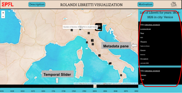
We used Javascript to code the visualisation, and for showing how the librettos are spread (or filtered) out we used the leaflet plugin with a slider for the time with interval of 22 years. We chose this specific interval of 22 years since the librettos were quite evenly spread out for each interval.

Every time, a user changes the interval, a mapping of all the librettos is dynamically regenerated, and if you hover over the marker, you could see the total number of librettos in that city. Also, once the user clicks on the city, a pane on the right (metadata pane) opens up which shows the metadata extracted for that time interval and city.

For each entry in the metadata pane, we show the following data (if extraction was successful):

• Title and link of the manifest it is related to
• Year
• Theatre Name
• Composer
• Genre and Occasion

This visualisation screenshot shows the initial overview for the librettos in 1804 and with the corresponding metadata pane, and markers for each city plotted.

If the user clicks on the city marker again, it zooms in to the city which shows where each extracted theatre is located.

Also, with every metadata pane entry, there might be a dropdown menu available for title or composer. This dropdown menu give the user an option to see links for 2 different types of metadata types:

• For a composer playing in different cities for a time interval of 22 years
• For a title being played in different cities for a time interval of 22 years

This visualisation screenshot shows the composer links for Pieter Metastasio in 1716 and links the five cities together. When the user hovers on the links, the users which plays were played in which year by the same composer.

Finally two buttons, Description: for providing a brief of what librettos are and the dataset we are using, and Motivation: what we doing with the libretti, are also added to provide context to our visualisation for an outside user. The code and the instructions to run the visualisation for local development are mentioned on Github.

Quality assessment

To evaluate our entity extraction we constructed evaluation metrics (e.g.: recall, precision) and we furthermore included in our visualization a link to the original documents. The link to the original document can be used by external users and by us to check the extracted entities by hand. Based on those metrics and our personal opinion (also given some hand checks with the linked source) we formulate the limitations and possible improvements of our project.

Metrics

In order to evaluate the results of our entity extraction we have to consider two conceptual metrics: 1) How many entities were we able to extract and 2) how correct are the extracted entities. The rate or number of extracted entities can be easily calculated by counting the numbers of extractions per group and dividing it by number of possible extractions (e.i. number of observations). The relative and absolute number of this retrieval rate are denoted in the table below:

Feature Extraction/Linking

Feature	Cities	Performance Location	Composer	Genre	Occasion	Performance Location Localization	Title MediaWiki Linking	Composer MediaWiki Linking
Relative	72.97%	76.21%	26.03%	95.04%	36.30%	42.16%	91.35%	23.87%
Absolute	810	846	289	1055	403	468	1014	265

This, however, does not tell us what percentage of the retrieved entities are correct. Therefore, in a second step, we analyze the percentage of our entities which are correctly identified by comparing it to a ground truth. To compute the ground truth, we randomly selected a subset of 20 librettos and extracted the correct entities by hand. By comparing our extracted entities with the correct entities, we can compute confusion matrices and metrics such as precision and recall. However, to calculate confusion matrices in this non binary case of entity extraction, we have to adjust the notation of the confusion matrix slight and adjust the definition of false negative, true positive, true negative, and false positive to our case. The adjusted notation is as follows:

Notation of Confusion Matrices

True Negative	Entity information not existing	No Extraction
False Negative	Entity information existing	No Extraction
False Positive	Entity information not existing Entity information existing	Something extracted Incorrect Extraction
True Positive	Entity information existing	Correct Extraction

Given this definition we can now proceed to calculate confusion matrices for selected entities:

City Extraction True Class Negative Positive Predicted Class Negative 0 7 Positive 1 12

Performance Location Extraction True Class Negative Positive Predicted Class Negative 5 3 Positive 2 10

Composer True Class Negative Positive Predicted Class Negative 16 3 Positive 0 1

Theater Localisation True Class Negative Positive Predicted Class Negative 10 6 Positive 0 4

By compiling confusion matrices for all our entities, we can calculate precision and recall metrics for the positively labeled entities. Recall in this sense is also referred to as sensitivity and precision as positive predictive values. Below a table shows the recall and precision rates for each feature extraction. The number on which the calculated metrics are based on is indicated in brackets.

Recall/Precision Feature Extraction and Linking

	Cities	Performance Location	Composer	Title	Genre	Occasion	City Localization	Performance Location Localization	Title MediaWiki Linking
Precision	92.3% (N=13)	83.3% (N=12)	100% (N=1)	80% (N=20)	100% (N=20)	100% (N=5)	100% (N=12)	100% (N=12)	66.6% (N=20)
Recall	63.2% (N=19)	77% (N=13)	25% (N=4)	100% (N=16)	100% (N=20)	100% (N=5)	100% (N=12)	0.44% (N=12)	77% (N=20)

Evaluation of Metrics

Before we interpret our evaluation metrics, we have to note that the size of our ground truth is very small. This is caused by the fact that the compilation of a ground truth is very labor and time intensive . The creation of our ground truth of twenty observations took us almost a day. The small size of our ground truth is problematic for the validity of some calculated metrics. Especially, the recall and precision metrics for some entities with a small number of observations are highly questionable. Therefore, in the following evaluation we will ignore any metrics which are based on less than 10 observations.

Looking at our calculated evaluation metrics we can deduce following:

• For all entities we reach a high precision moving in a range of at least 80% to at most 100%. Given that one of our main objectives is to produce reliable data and to correctly extracted entities, this is a very good sign. However, optimally we would like to further improve our precision.

• The recall of our entity extraction is lower than our precision. We could improve on this by further including more complex extraction models and by obtaining a better OCR quality of the coperte.
• The number of entities which don't exist can be quite high as for example in the case of composers, occasions or theaters

• Depending on the data source (coperta or title) the recall seems to vary, this is probably due to the low OCR quality we obtained.

Limitations and possible improvements

Considering our evaluation metrics and our personal opinion, we could certainly improve on our entity extraction. In particular we identified following topis on which we could improve or by which we are limited:

• OCR Quality: Looking at the recall of the information extracted from the coperta and considering our personal experience while working on the data, we were limited to a certain amount by the OCR quality. The OCR qulaity produced by Tesseract was not always sufficient to reach the quality of our extraction which we would like to have. Experiments with OCR sowftware as Adobe OCR or Google Vision would possibly improve our extraction potential.

• Data Limitations: In certain cases it was very difficult to extract or link data, because either the data we wanted extract didn't exist (theater names, Composer names) or the name of for example Theaters chaanged over time.

• Additional Sanity Check of extractions: We furthermore could certainly improve on our extraction algorithms. Here we would have to continuously evaluate the performance of algorithms and try to adapt to the mistakes made by our extraction pipeline.

• Limited generalization of algorithms: For some of the extraction such as for composer, we used regular expression based on the patterns seen in the data. This data is limited and if new data arrives with new patterns, the algorithm might need to slightly evolve to scale to all the librettos.

• Improvements for visualization: If all the librettos are available and are needed to be visualized, the existing visualization pipeline would need to include concepts like tiling so that the data loading part is not slow and can only be done for the part the user is interested in seeing.

Planning

The draft of the project and the tasks for each week are assigned below:

Weekly working plan

Timeframe	Task	Completion
Week 4
07.10	Evaluating which APIs to use (IIIF)	✅
	Write a scraper to scrape IIIF manifests from the Libretto website
Week 5
14.10	Processing of images: apply Tessaract OCR	✅
	Extraction of dates and cleaned the dataset to create initial DataFrame
Week 6
21.10	Design and develop initial structure for the visualization (using dates data)	✅
	Running a sanity check on the initial DataFrame by hand
	Matching list of cities extracted from OCR using search techniques
Week 7
28.10	Remove irrelevant backgrounds of images	✅
	Extract age and gender from images
	Design data model
	Extract tags, names, birth and death years out of metadata
Week 8
04.11	Get coordinates for each city and translation of city names	✅
	Extracted additional metadata (opera title, maestro) from the title of Libretto
	Setting up map and slider in the visualization and order by year
Week 9
11.11	Adding metadata information in visualization by having information pane	✅
	Checking in with the Cini Foundation
	Preparing the Wiki outline and the midterm presentation
Week 10
18.11	Compiling a list of musical theatres	✅
	Getting better recall and precision on the city information
	Identifying composers and getting a performer's information
	Extracting corresponding information for the MediaWiki API for entities (theatres etc.)
Week 11
25.11	Integrate visualization's zoom functionality with the data pipeline to see intra-level info	✅
	Linking similar entities together (which directors performed the same play in different cities?)
Week 12
02.12	Serving the website and do performance metrics for our data analysis	✅
	Communicate and get feedback from the Cini Foundation
	Continuously working on the report and the presentation
Week 13
09.12	Finishing off the project website and work, do a presentation on our results	⬜️

Links

• Github
• Website