Alignment of XIXth century cadasters: Difference between revisions
| Line 163: | Line 163: | ||
- [ ] And still time consuming and need close supervision => change of paradigm | - [ ] And still time consuming and need close supervision => change of paradigm | ||
<!-- | |||
After this liminary result, a lot of question were nevertheless still to be answered. For example, is the orientation of our maps precisely in the North direction ? Will it be possible to have an explicit order of maps reattachment ? Will the matching score be as good in the countryside as it was in the city ? Is the scale homogenous within an entire city ? Or what criteria could be used to automatise the template selection ? | After this liminary result, a lot of question were nevertheless still to be answered. For example, is the orientation of our maps precisely in the North direction ? Will it be possible to have an explicit order of maps reattachment ? Will the matching score be as good in the countryside as it was in the city ? Is the scale homogenous within an entire city ? Or what criteria could be used to automatise the template selection ? | ||
--> | |||
== AlignmentTool == | == AlignmentTool == | ||
Revision as of 18:34, 20 December 2021
Introduction
TODO: Examples of references (APA style)[1].
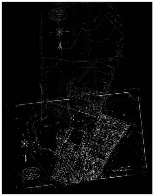
About a thousand of French napoleonian cadasters have been scanned and need from now to be aligned. A lot of different cities are included in this catalogue as La Rochelle, Bordeaux, Lyon, Lille, Le Havre and also cities that are no longer under French juridiction as Rotterdam.
Similarly to the work that had been done by the Venice Time Machine project, the idea is to attach every maps from a cadaster in order to get a single map of each city.
The main challenge for this project is the automatisation of this process, despite all inconsistencies in the maps, in terms of scale, orientation or conventions. Even if the instructions for the realisation of the maps were quite strict, some differences might last, for example in the scale, if there were nothing to show in some areas, or maps are not always oriented top-north (which is even not always indicated).
Deliverables
- [ ] Tool
   - [ ] rectification
   - [ ] Alignment
   - [ ] JSON generation
   - [ ] reconstruction of covered areas
- [ ] PoC: La Rochelle downtown
This project provides an exploration of possible automation for aligning cadastres, as well as the development of an interface (in the form of a Jupyter Notebook) to supervise this task.
Project setup
Methods exploration on Berney's cadaster
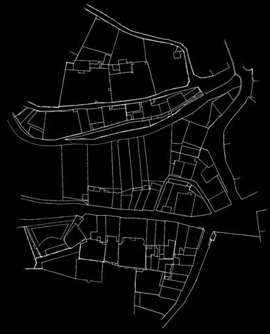
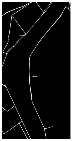
For the primary research of methods to reattach cadastral maps, the so called cadastre Berney from Lausanne (1827) has been used, as long as the ground truth for this particular case is known and lot of processing steps (as lines and classes predictions) have already been made. The first exercise has been made on the two first maps, using the lines prediction files. The quandary was to be able to detect the common parts of these two maps, in this case the Rue Pépinet and the top of Rue du petit chêne. Many different methods have been tested for that task, mainly with help of the openCV python library. The researches have focused on scale invariant feature transform (SIFT), General Hough Transform (GHT)[2] and Template Matching (TM).
Template matching principle
[ ] talk about the different matching modes: https://docs.opencv.org/4.x/df/dfb/group__imgproc__object.html#ga3a7850640f1fe1f58fe91a2d7583695d
[ ] define the score (at least for the mode used: cv.TM_CCOEFF_NORMED)
Template matching is an OpenCV[1] function provided under the name cv.matchTemplate(). It takes as an imput a large scale image and smaller one, called template, that it will try to find in the first image. Concretely, the function slides the template through the initial image and for each position, gives a score of closeness. Note that the template always fully overlap the image, therefore the template must be fully included in the image. The function gives then as an output a matrix with score for each position. It then easy to find the position of the best score.
This function is known to have better results on greyscale images. It is therefore a wise decision to apply it on the lines detected files.
First reattachment of two cadastral maps
The method that gave the most satisfying results (in terms of final output and computation time) was the template matching. The strategy is to cut a template in one of the maps and find the best match in the other one. Attaching the two maps together is then an almost straightforeward task, as long as the lines prediction files are only black (0) or white (255) pixels, and the final result is just the sum of the two of them adapted with the best matching position.
Lorem ipsum dolor sit amet, consectetur adipiscing elit, sed do eiusmod tempor incididunt ut labore et dolore magna aliqua. Ut enim ad minim veniam, quis nostrud exercitation ullamco laboris nisi ut aliquip ex ea commodo consequat. Duis aute irure dolor in reprehenderit in voluptate velit esse cillum dolore eu fugiat nulla pariatur. Excepteur sint occaecat cupidatat non proident, sunt in culpa qui officia deserunt mollit anim id est laborum.
Challenges Identification / Problem statement
[ ] Template extraction
[ ] Orientation/scale
[ ] Growth
[ ] Good coherence metric, aligned with human understanding
Organisation
[ ] merge
Timeline summary of first steps
| Matching method | Template extraction | Growth | |
|---|---|---|---|
| Week 4 | SIFT | - | 1 to 1 |
| Week 5 | SIFT and GHT | Manual | 1 to 1 |
| Week 6 | GHT and TM | Manual | semi-automated 1 to 1 |
| Week 7 | GHT and TM | Manual | semi-automated 1 to 1 |
| Week 8 | TM | Manual and along lines | semi-automated 1 to 1 |
| Week 9 | TM | Manual and along lines | 1 to 1 or N |
| Week 10 | TM | Manual and along lines | 1 to 1 or N |
Final milestones of semester
| Objective | |
|---|---|
| Week 11 | Extract lines on a first set of cadastral maps (La Rochelle or Bordeaux) & manage pipeline |
| Week 12 | Test pipeline on the new extracted lines files |
| Week 13 | Adapt our model or extend it on other cities |
| Week 14 | Final presentation |
Automatisation process
In order to automate the alignment task, efforts where put in three of the main challenges identified. A pipeline was then built to automatically extract templates, take into account variations in scales and orientations and iteratively spread over adjacent cadastres to cover large areas. However the incapacity to meet the fourth challenge, defining a semantically coherent metric, hindered the generalisation of this approach and led to mixed results.
This exploration was undertook on the lines pre-extracted from Berney's 1827 cadastres of Lausanne.
Automatic template extraction
In cadastres, the overlapping areas are situated on the borders of the maps. Hence, the template extraction process was automated to extract templates around most excentric points along given lines that still coded for a line.
To do so, an imaginary path parametrised by an angle is drawn from the center of the cadastre to its edge. Pixels values along this path are extracted and used to retrieve the coordinates of the last non-zero pixel value (ie. extracted line on the cadastre). A template can then be extracted around this point.
The function automating this task takes an integer N as argument that defines the number of templates to be extracted. Templates are then extracted along paths parametrised by the linear division of the circle in N pieces (see extract_templates). Examples are shown in the left hand side plot present in the figure on the right.
Nevertheless these plot mainly highlight the fragility of the matching method. Indeed they underline that the TM score doesn't align with the human understanding of the problem. Moreover, as TM is highly dependent on the templates, this approach is highly dependent on the chosen number of extracted templates N. For example here extracting 9 templates resulted in a coherent best match but extracting one less template yielded wrong results.
Orientation and scale integration
One of the factor deteriorating the quality of the matches are the slight variations of orientation. Thus, in order to limit this influence (and potentially to prepare to non-oriented cadastres) the matching process was made orientation invariant (over a given discrete range). The same procedure was applied to scales as Lausanne's cadastres relative scales are mixed between 1:1 and 1:2 (or inversly 1:0.5). The matching process was then a grid-search over the specified angles and scales, with scores obtained by matching the extracted template on the modified (rotated and rescaled) target cadastre.
However, beside increasing the computational cost, multiplying the number of parameters also heightens the chance of semantically incoherent match to get the best score (as there is only one, or few, good match and all others are deceiving).
NB.: at this state of the project, this method was achieved by rescaling and rotating the whole target cadastre. This approach is largely suboptimal and computationally very expensive, it was changed afterwards (as described here).
Peripheral growth
- Iterative growth with successive anchors 001, 009, 010 and 008. Taking into account slight variations in orientation and two scales.
Limitations
Due to these limitations, we decided to shift paradigm and to develop a tool more closely supervised.
- [ ] Trials
   - [ ] Automatic template extraction
   - [ ] Adjacent cadastres considerations: iterative growth
   - [ ] Taking into account: both orientation and scale
- [ ] Low computational Efficiency
- [ ] Necessity to fine-tune manually parameters due to the lack of a metric closer to human understanding
- [ ] Sometimes poor results (eg. less dense areas, etc.)
- [ ] Too fragile method ?
- [ ] And still time consuming and need close supervision => change of paradigm
AlignmentTool
[ ] Jupyter Innotater
[ ] Rectifying
   [  ] rotation
   [  ] name
   [  ] NOT IMPLEMENTED: scale
[ ] Matching process
   [  ] template selection
   [  ] target selection
   [  ] orientation dependent or not
[ ] Output = "raw" network
[ ] Rebuilding
   [  ] homographies
   [  ] pairwise visualisation
   [  ] area growth
      [  ] new network
      [  ] inverse homographies included
      [  ] shortest path
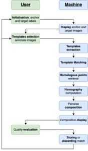
The AlignmentTool was developed to offer a highly supervised method to perform the cadastres' alignment.
The backend processes are mainly handled through OpenCv[1], the data structure is managed with NetworkX[3], and the Notebook interface relies on jupyter-innotater[4]. The architecture and proceeding of each of these components are detailed below. Finally, the results of the proof of concept undertook on La Rochelle intramural Napoleonic cadastres from 1811 are described and illustrated.
Backbone
The development of this tool compelled us to slightly revise the conceptual and theoretical framework for the matching and composition processes. The three major steps consisting in homologous points retrieval, pair-wise transformations computation and propagation are described in this section.
Matching
The matching model aims at finding two pairs of homologous points in the anchor and target cadastres (see get_target_homologous). It relies on TM (described above). On the anchor cadastres the tagged positions are the top-left and bottom-right corners of the extracted template. On the target one, the corresponding points are retrieved from the best match found.
If both of the cadastres share the same orientation (ie. matches are evaluated without taking into account additional rotations), then the pixel associated with the top-left corner of the template corresponds to the location with the highest value computed through TM and the pixel associated with the bottom-right corner is given by adding the template width and height.
If both of the cadastres don't share the same orientation, this task requires slightly more efforts. This procedure iteratively rotates the template, resulting in images of different shapes filled with void, and performs TM using these rotated templates (see orientation_matching). Thus, the coordinates of the best match will correspond to the top-left corner of the best rotated template, which is no longer in line with the top-right corner of the extracted template. The new pixel coordinates corresponding to the orignial template top-left and bottom-right corners are retrieved by artificially rotating the original template and computing the displacement of specified points (see shift_template).
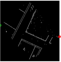
An example of points tracking in the rotated templates is shown on the figure on the right. The figure below displays the results obtained through this method on a pair of non-aligned cadastres.
Homography
Homographies are transformation matrices (3 by 3), widely used in computer vision, mapping points in one image to corresponding ones in another image. In the context of this project, homographies are restricted to Euclidean transformations (allowing rotations and translations but preserving the distance between every pair of points). However, as the rest of the implementation is more general, slight modifications of the homographies' computation could enable the intergration of more complex transformations (eg. affine or projective) within the pipeline.
The pairs of homologous points retrieved through the matching process allows to compute the corresponding homography between the anchor and target cadastres. On both images the pair of coordinates define a vector from the top right to the bottom left tags. As they are considered to refer to the same geographic entity, the cadastres can be re-oriented (relatively to one another) by calculating the angle α between these vectors. The translations in 𝑥 and 𝓎 are computed by comparing points corresponding to the top left corner in the anchor image and target one (after re-orientation). The homography matrix is then given by:
This process is encoded in the function vector_alignment. It allows to turn the matches characterised by two pairs of homologous points into a transformation matrix, which can be applied on the target cadastre to obtain its composition with its anchor through warpTwoImages based on cv2.warpPerspective.
Propagation
Homographies demonstrate convenient properties that allow to propagate pairwise homographies in order to reconstruct larger areas.
- Inversion — If H1,2 is known, then H2,1 is given by the inverse of H1,2
Allows to get rid of the directionality of the graph - Composition — If H1,2 and H2,3 are known, then H1,3 is given by the product of H1,2 and H2,3
Allows to directly link each connected nodes to each others
Thus, taking benefits of the network structure of the data (descibed below), the pairwise homographies can be operated to recover whole areas.
This procedure is done by building a new graph centered on a selected node, and linked to every node that was connected to it in the original network (without notion of directionality). All other nodes are only connected (as targets) to this central node.
Each one of the edges is characterised by an homography between the central node (anchor) and the connected component (target). These homographies are computed as the product of pair-wise homographies along the shortest path linking the selected central node to the target in the original graph (see buildCenteredNetwork).
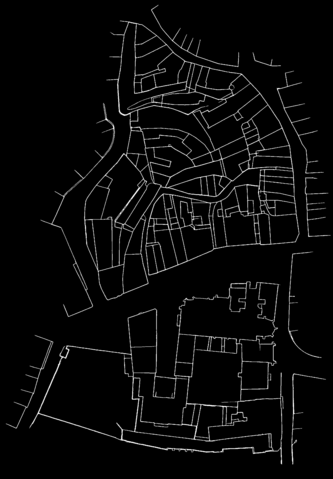
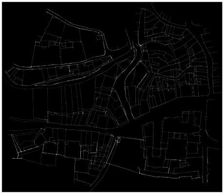
The two images below show an example of cadastres composition, either using direct match (left) or homographies propagation along a path in the network (right).
- Alignment of cadastres with direct edge or through propagation.
Network structure
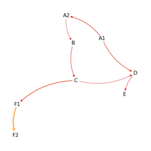
The matches (when selected by the user) are collected in a directed graph. The nodes are the cadastres (or their labels) and the edges link the anchors (cadastres within which templates have been extracted) to their targets (cadastres matched). The edges store information about the matches between anchors and targets: their score and informations related to the matched positions (top left and bottom right corners of the extracted template in the anchor and corresponding positions in the target). An exemple of a possible realisation of such graph (for La Rochelle, 1811) is shown below.
These graph can be saved in JSON format with the following generic structure:
{
    "directed": true,
    "multigraph": false,
    "graph": {},
    "nodes": [{
        "h": int — height of the corresponding image,
        "w": int — width of the corresponding image,
        "label": str — name
    }, {
        "h": int — height of the corresponding image,
        "w": int — width of the corresponding image,
        "label": str — name
    }],
    "match": [{
        "score": float — score of the template matching process,
        "anchor_tl": tuple: two int — coordinate of the template top left corner on the anchor,
        "anchor_br": tuple: two int — coordinate of the template bottom right corner on the anchor,
        "target_tl": tuple: two int — coordinate corresponding to anchor_tl on target,
        "target_br": tuple: two int — coordinate corresponding to anchor_br on target,
        "anchor": str — name of the anchor cadastre\node,
        "target": str — name of the target cadastre\node
    }]
}
User guide
Rectification
Template Selection
Network Analysis
Composition visualisation
PoC
Lines detection process
Discussion and limitations
- [ ] Lack of convincing metric / purely qualitative results
- [ ] Failing to automate the task
Why doesn't it work ?
Future Work
- [ ] Tool roadmap
   - [ ] Integration of other matching methods
   - [ ] Integration of more automation (adjacent matching)
   - [ ] improve UX
- [ ] Taking into account matches from all adjacent cadastres and recursive adjustments
   - [ ] eg. Bundle Adjustment[5]
- [ ] Automation
   - [ ] more heuristic and domain knowledge — in traditional ML/CV methods
   - [ ] investigate "deeper" approaches => add some literature: eg. [6] [7]
- [ ] Alignment on Openstreetmap
References
- ↑ 1.0 1.1 1.2 Bradski, G. (2000). The OpenCV Library. Dr. Dobb's Journal of Software Tools. User site: https://opencv.org
- ↑ Ballard, D. H. (1981). Generalizing the Hough transform to detect arbitrary shapes. In Pattern Recognition (Vol. 13, Issue 2, pp. 111–122). Elsevier BV. doi:10.1016/0031-3203(81)90009-1
- ↑ Aric A. Hagberg, Daniel A. Schult, & Pieter J. Swart (2008). Exploring Network Structure, Dynamics, and Function using NetworkX. In Proceedings of the 7th Python in Science Conference (pp. 11 - 15). Documentation: https://networkx.org/documentation/stable
- ↑ Lester, D (danlester). (2021). jupyter-innotater. GitHub Repository: https://github.com/ideonate/jupyter-innotater.
- ↑ Brown, M., & Lowe, D. G. (2007). Automatic panoramic image stitching using invariant features. International journal of computer vision, 74(1), 59-73. doi:10.1007/s11263-006-0002-3
- ↑ Sun, K., Hu, Y., Song, J., & Zhu, Y. (2021). Aligning geographic entities from historical maps for building knowledge graphs. International Journal of Geographical Information Science, 35(10), 2078-2107. doi:10.1080/13658816.2020.1845702
- ↑ Duan, W., Chiang, Y.Y., Knoblock, C., Jain, V., Feldman, D., Uhl, J., & Leyk, S. (2017). Automatic Alignment of Geographic Features in Contemporary Vector Data and Historical Maps. In Proceedings of the 1st Workshop on Artificial Intelligence and Deep Learning for Geographic Knowledge Discovery (pp. 45–54). Association for Computing Machinery. doi:10.1145/3149808.3149816
