Data Ingestion of Guide Commericiale: Difference between revisions
| (47 intermediate revisions by 3 users not shown) | |||
| Line 128: | Line 128: | ||
=== Deliverable 1: Full ingestion pipeline === | === Deliverable 1: Full ingestion pipeline === | ||
The final pipeline consists of 2 executable Python scripts ( | The final pipeline consists of 2 executable Python scripts (main.py and conll2002toCsv.py), 1 Python notebook to handle the cleaning and formatting of the data obtained from the semantic annotation process (cleaning&formatting.ipynb), and a trained semantic annotation model. A user will be able to pass the relevant sections of the scanned pdf of 1853 Guida Commerciale through main.py, which will perform text extraction and automatic formatting, outputting a series of text files that correspond to each scanned page. These text files should then be imported into INCEpTION, in which a user can use a pre-trained model to analyze and extract labels to each text file. This will output CONLL 2002 files for each page, which is then converted into a CSV file with the conll2002toCsv.py Python script. This will output a CSV file, with each line as a row, each annotation as a column, and the relevant annotated text as a field in the CSV. This CSV can be passed into cleaning&formatting.ipynb, which will clean the data and map it onto a GeoJSON file, as well as onto an old map of Venice. | ||
=== Deliverable 2: | === Deliverable 2: Diagnostics dashboard === | ||
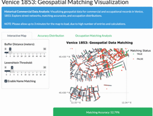
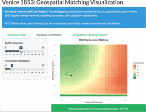
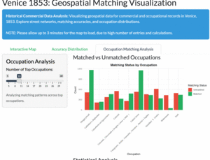
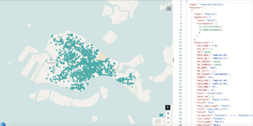
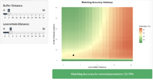
Analysis of the output of the ingestion pipeline will take the form of a dashboard (Shiny R App) that will display the accuracy of the ingestion pipeline by comparing how many of the points in the 1853 guide commercial lined up with points from the 1808 guide commercial by street name and by geometric location. The map will display points correctly plotted in green, and those incorrectly plotted in red. There is also an option to remove the name matching, so that the accuracy is evaluated purely based on geometric location. The size of the error allowed can be adjusted by the user. Diagnostic plots, such as a heatmap the possible distributions of accuracy, are also supplied, as well as the distribution of different occupations and the percentage of which were matched. This includes statistical tests including post hoc tests that can be adjusted by the user for further analysis. | Analysis of the output of the ingestion pipeline will take the form of a dashboard (Shiny R App) that will display the accuracy of the ingestion pipeline by comparing how many of the points in the 1853 guide commercial lined up with points from the 1808 guide commercial by street name and by geometric location. The map will display points correctly plotted in green, and those incorrectly plotted in red. There is also an option to remove the name matching, so that the accuracy is evaluated purely based on geometric location. The size of the error allowed can be adjusted by the user. Diagnostic plots, such as a heatmap the possible distributions of accuracy, are also supplied, as well as the distribution of different occupations and the percentage of which were matched. This includes statistical tests including post hoc tests that can be adjusted by the user for further analysis. | ||
{|class="wikitable" style="margin: 1em auto 1em auto;" | {|class="wikitable" style="margin: 1em auto 1em auto;" | ||
|[[File:fdh_dashboard_map.gif|300px|thumb|center| | |[[File:fdh_dashboard_map.gif|300px|thumb|center|'''Figure 1a''': Interactive dashboard]] | ||
|[[File:fdh_dashboard_heatmap.gif|300px|thumb|center| | |[[File:fdh_dashboard_heatmap.gif|300px|thumb|center|'''Figure 1b''': Diagnostic heatmap showing distribution of accuracies]] | ||
|[[File:fdh_dashboard_barplot.gif|300px|thumb|center| | |[[File:fdh_dashboard_barplot.gif|300px|thumb|center|'''Figure 1c''': Diagnositc barplot and significance tests showing differences in matched points]] | ||
|} | |} | ||
| Line 145: | Line 145: | ||
== Approach 1: General == | == Approach 1: General == | ||
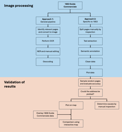
[[File:Flowchartforwiki.png|thumb|right|400px|Figure | [[File:Flowchartforwiki.png|thumb|right|400px|'''Figure 2''': flowchart of modelling methodology]] | ||
=== Pipeline Overview === | === Pipeline Overview === | ||
| Line 191: | Line 191: | ||
# Clean and format data | # Clean and format data | ||
## Logical segmentation | ## Logical segmentation | ||
## Handling rows with multiple | ## Handling rows with multiple parish and street values | ||
## Handling rows with multiple names | ## Handling rows with multiple names | ||
## Occupation broadcasting | ## Occupation broadcasting | ||
| Line 200: | Line 200: | ||
=== Find page ranges of interest === | === Find page ranges of interest === | ||
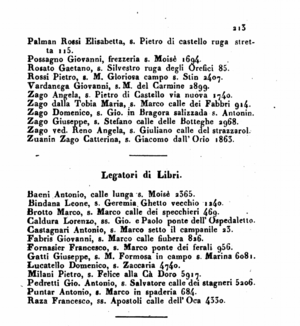
[[File:pages_of_interest.png|300px|thumb|right|'''Figure 3''': Page of interest]] | |||
The key difference with this approach compared to approach 1 was that instead of relying on a program to group our pages, we manually went through our document and found a range of pages that were of interest to us. This allowed us to go into the next steps of our pipeline with confidence, knowing we don't need to deal with the uncertainty of whether our page had irrelevant data or not. | The key difference with this approach compared to approach 1 was that instead of relying on a program to group our pages, we manually went through our document and found a range of pages that were of interest to us. This allowed us to go into the next steps of our pipeline with confidence, knowing we don't need to deal with the uncertainty of whether our page had irrelevant data or not. | ||
| Line 215: | Line 216: | ||
After performing the annotations and obtaining a CONLL 2002 file for each page in the 1853 Guida Commerciale on which we performed text extraction, we converted the CONLL 2002 files into a single CSV file using conll2002toCsv.py to further clean and format the data. | After performing the annotations and obtaining a CONLL 2002 file for each page in the 1853 Guida Commerciale on which we performed text extraction, we converted the CONLL 2002 files into a single CSV file using conll2002toCsv.py to further clean and format the data. | ||
The resulting CSV file is loaded into a Pandas DataFrame. After this, duplicate rows in the DataFrame are dropped to ensure we have unique entries. After this, we set up a contextual order for each row, starting from the "FIELD" and "OCC" tags (representing occupations) and ending with the "NUM" tag (representing the door number) and reordered the DataFrame in this order. The specific order for entries is "["FIELD", "OCC", "LAST_N", "FIRST_N", "PER_TITLE", "PER_GRP", "PER_COMPL", "LOC_ISLA", "LOC_STR", "LOC_PAR", "NUM"]". | The resulting CSV file is loaded into a Pandas DataFrame. After this, duplicate rows in the DataFrame are dropped to ensure we have unique entries. After this, we set up a contextual order for each row, starting from the "FIELD" and "OCC" tags (representing occupations) and ending with the "NUM" tag (representing the door number) and reordered the DataFrame in this order. The specific order for entries is "["FIELD", "OCC" (occupation), "LAST_N", "FIRST_N", "PER_TITLE", "PER_GRP", "PER_COMPL", "LOC_ISLA", "LOC_STR" (street), "LOC_PAR" (parish), "NUM" (house number)]". | ||
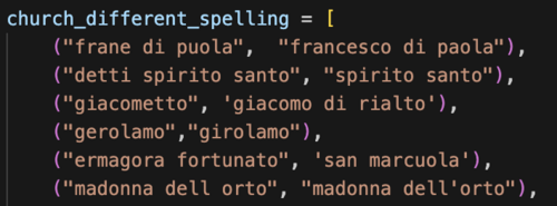
[[File:spelling_fix.png|500px|thumb|right|'''Figure 4''': Example of equivalent spellings for the same parish]] | |||
Next, we perform two rounds of logical segmentation, iterating over rows of the Pandas DataFrame and attempting to reconcile rows with incomplete or logically segmented data. This merges rows where address components such as | Next, we perform two rounds of logical segmentation, iterating over rows of the Pandas DataFrame and attempting to reconcile rows with incomplete or logically segmented data. This merges rows where address components such as house number, street, and parish are split across multiple rows. Any empty or redundant rows are removed after merging. This process ensures that logically connected segments are consolidated into a single row. | ||
Following this, we refine the segmentation process by addressing rows with multiple | Following this, we refine the segmentation process by addressing rows with multiple parish and street values. Since these are logical components of an address, we ensure these fragmented components are correctly associated with their respective entries. | ||
Then, we handle cases with multiple individuals or names associated with a single entry. This ensures that all information related to individuals or groups of individuals is consolidated into a single row in the Pandas DataFrame. | Then, we handle cases with multiple individuals or names associated with a single entry. This ensures that all information related to individuals or groups of individuals is consolidated into a single row in the Pandas DataFrame. | ||
| Line 225: | Line 228: | ||
The next step involves Occupation Broadcasting. In this step, we focus on broadcasting occupation information down to subsequent rows where it is missing, as long as the previous entry has a valid occupation entry. This ensures that every relevant entry has an occupation associated with it. This is an important step because the 1853 Guida Commerciale lists the occupation once and then lists all the individuals who work in that specific occupation. | The next step involves Occupation Broadcasting. In this step, we focus on broadcasting occupation information down to subsequent rows where it is missing, as long as the previous entry has a valid occupation entry. This ensures that every relevant entry has an occupation associated with it. This is an important step because the 1853 Guida Commerciale lists the occupation once and then lists all the individuals who work in that specific occupation. | ||
Another important step is cleaning the | Another important step is cleaning the parish values to ensure we can accurately map the entries to their respective districts based on the parish-to-district dictionary. Some common discrepancies and errors exist due to the text extraction process, such as spelling mistakes and inaccurate text extraction. In addition to this, parishes and churches have different spellings that must be accounted for when a parish is extracted from PDFPlumber. Common errors also include inconsistent abbreviations such as "s .", "s.", "S .", "ss .", etc., were removed from the parish value. In addition to this, we ensured all parishes were in lowercase and stripped of any trailing spaces. After this, we added another column to represent the district and applied the existing parish-to-district dictionary to ensure all the parishes with corresponding values were mapped. | ||
=== Plot on a Map === | === Plot on a Map === | ||
| Line 281: | Line 280: | ||
|- | |- | ||
|} | |} | ||
<p>'''Table 1''' | <p>'''Table 1''' Text extraction accuracy measures.</p> | ||
</div> | </div> | ||
Looking at the performance of our text extraction on five randomly chosen pages, we manually cross-checked every word on these pages against the original document, and counted the number of errors we found. As for the heuristic of what constitutes as an error, the criteria goes as follows: | Looking at the performance of our text extraction on five randomly chosen pages, we manually cross-checked every word on these pages against the original document, and counted the number of errors we found. As for the heuristic of what constitutes as an error, the criteria goes as follows: | ||
* If a word does not show up as it is in the original document, it counts as | * If a word does not show up as it is in the original document, it counts as 1 error. | ||
* If 4 words are clumped together in the PDFPlumber when they should have spaces in between, this counts as 4 errors. | * If 4 words are clumped together in the PDFPlumber when they should have spaces in between, this counts as 4 errors. | ||
* If any marks are generated that were not intentionally in the old document, that counts as 1 error. | * If any marks are generated that were not intentionally in the old document, that counts as 1 error. | ||
| Line 293: | Line 292: | ||
Most errors were due to certain words being hand written too closely together, and then the OCR done by Google analyzed them to be together when they should be two distinct words. Similarly, certain commas were written slightly too far from the word, leading to the OCR separating the comma from the word it should be in front of. Only two of these errors were due to a letter being misinterpreted, giving us good confidence that the OCR was reliable. | Most errors were due to certain words being hand written too closely together, and then the OCR done by Google analyzed them to be together when they should be two distinct words. Similarly, certain commas were written slightly too far from the word, leading to the OCR separating the comma from the word it should be in front of. Only two of these errors were due to a letter being misinterpreted, giving us good confidence that the OCR was reliable. | ||
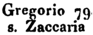
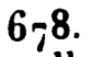
The figures below show examples of the errors we saw during our measuring process. | The figures below show examples of the errors we saw during our measuring process. '''Figure 5a''' and '''5b''' show the two times that the OCR misinterpreted a character and gave an output that was different from the actual document. In '''5a''' TODO, the "g" above the "Z" extended in a way where it was read as "Ž", and in '''5b''', the "7" was written so low that the OCR read it as a dash ("-"). As for '''Figure 5c''', even though it might not look too close to the human eye, the OCR interpreted these two words to be too close to each other, resulting in "s.Martino" instead of the correct "s. Martino". | ||
{|class="wikitable" style="margin: 1em auto 1em auto;" | {|class="wikitable" style="margin: 1em auto 1em auto;" | ||
|[[File:Weird_z.png|300px|thumb|center| | |[[File:Weird_z.png|300px|thumb|center|'''Figure 5a''': Z read as "Ž"]] | ||
|[[File:678.png|300px|thumb|center| | |[[File:678.png|300px|thumb|center|'''Figure 5b''': 7 read as "-"]] | ||
|[[File:together.png|300px|thumb|center| | |[[File:together.png|300px|thumb|center|'''Figure 5c''': Words being too close together]] | ||
|} | |} | ||
| Line 343: | Line 342: | ||
|- | |- | ||
|} | |} | ||
<p>'''Table 2''' Semantic | <p>'''Table 2''' Semantic annotation accuracy measures.</p> | ||
</div> | </div> | ||
Looking at the performance of this model on five randomly chosen manually cleaned up pages from our text extraction process, we manually checked each token on these pages, and counted the number of errors we found. As for the heuristic of what constitutes as an error, the criteria goes as follows: | Looking at the performance of this model on five randomly chosen manually cleaned up pages from our text extraction process, we manually checked each token on these pages, and counted the number of errors we found. As for the heuristic of what constitutes as an error, the criteria goes as follows: | ||
| Line 353: | Line 352: | ||
As we can see from the total accuracy, the semantic annotation worked well on randomly sampled pages. A key note to make here is that no one in our team speaks Italian, possibly resulting in further errors that we were not able to verify without extensive work. | As we can see from the total accuracy, the semantic annotation worked well on randomly sampled pages. A key note to make here is that no one in our team speaks Italian, possibly resulting in further errors that we were not able to verify without extensive work. | ||
=== Mapping accuracy === | === Mapping accuracy === | ||
| Line 370: | Line 362: | ||
==== Error 1: Failure to Map ==== | ==== Error 1: Failure to Map ==== | ||
First, it is important to understand the total number of entries that need mapping. To do so, we review the process of data cleanup and how that impacts the number of entries. Initially, the CSV file had 4357 entries, which was reduced to 4346 entries after dropping duplicate entries. After the first and second rounds of logical segmentation, we have 3811 and 3769 entries, respectively. After handling multiple | First, it is important to understand the total number of entries that need mapping. To do so, we review the process of data cleanup and how that impacts the number of entries. Initially, the CSV file had 4357 entries, which was reduced to 4346 entries after dropping duplicate entries. After the first and second rounds of logical segmentation, we have 3811 and 3769 entries, respectively. After handling multiple street and parish values in one entry, we have 3696 entries. After handling multiple people in one entry, we have 3642 entries. After completing occupation broadcasting, we have 3604 entries. Finally, after performing other miscellaneous cleaning and parish/church reconciliation, we still have 3604 entries. Of the 3604 entries, 3602 entries have an occupation value. Some other interesting findings that showcase the limitations of the semantic annotation and PDFPlumber text extraction are that only 3486 entries have a last name, and 3395 entries have a first name. In addition to this, 3365 entries have a first and last name. Another interesting finding is that 3412 entries have a parish value. | ||
[[File:Mapped_points.png|500px|thumb|right|'''Figure 6''': Large number of entries were plotted on the map despite existing errors]] | |||
During the initial phase of mapping parishes to district values, we realized that 645 entries with a parish value did not map to a district. During this process, we noticed some errors with our data cleaning as our cleaning step did not account for “m formosa” (136 entries), “m gloriosa” (94 entries), etc. They refer to “maria formosa” and “maria gloriosa dei frari” respectively. After manually inspecting the entries that did not map, we changed our cleaning and formatting steps to improve the % of parishes that are mapped to a district. After making fixes, we increased the % of entries with a parish that maps to a dictionary from 81.09% (2767 entries mapped) to '''95.78%''' (3268 entries mapped). | During the initial phase of mapping parishes to district values, we realized that 645 entries with a parish value did not map to a district. During this process, we noticed some errors with our data cleaning as our cleaning step did not account for “m formosa” (136 entries), “m gloriosa” (94 entries), etc. They refer to “maria formosa” and “maria gloriosa dei frari” respectively. After manually inspecting the entries that did not map, we changed our cleaning and formatting steps to improve the % of parishes that are mapped to a district. After making fixes, we increased the % of entries with a parish that maps to a dictionary from 81.09% (2767 entries mapped) to '''95.78%''' (3268 entries mapped). | ||
| Line 389: | Line 383: | ||
* 21 cases for "gio battista in bragora" and 7 cases for "gio battista" — corrected to "giovanni battista in bragora" and mapped to Castello. | * 21 cases for "gio battista in bragora" and 7 cases for "gio battista" — corrected to "giovanni battista in bragora" and mapped to Castello. | ||
Following these manual corrections, only 4.22% (n = 144) of the data remained unmappable. These remaining errors were due to major spelling errors that occurred once. For time's sake, we avoided fixing 144 specific mistakes and wanted to showcase some errors due to text extraction and semantic annotation. | Following these manual corrections, only 4.22% (n = 144) of the data remained unmappable. These remaining errors were due to major spelling errors that occurred once. For time's sake, we avoided fixing 144 specific mistakes and wanted to showcase some errors due to text extraction and semantic annotation. | ||
Some other interesting statistics are that we had 3093 entries with a house number and district and 3227 entries with a house number and parish. At the end of the pipeline, 3469 points were plotted. At first, this may seem alarming. However, after inspecting the existing single-door GeoJSON, we realized there are multiple entries with the same house number, district, first name, last name, occupation, parish, etc., as house numbers can be divided further into segments such as A, B, C, etc. In our model, we only merge the overall house number and district. As such, we plot a larger number of points. After further analyzing these points, we discovered that there are 501 unique duplicate entries. When summed up, this leads to 1304 total duplicate entries, as each unique duplicate entry can have multiple duplicates. Therefore, the extra number of entries that are plotted is equal to 803. Therefore, the total number of points/entries plotted is 2666. For all entries with a house number and district, 86.19% (accuracy) of them were plotted on the map. For all entries with a house number and parish, 82.61% (accuracy) of them were plotted. This discrepancy exists because not all parishes were mapped to the district. Of all the entries, including those without a parish, district, occupation, or house number value, '''73.9%''' are plotted | Some other interesting statistics are that we had 3093 entries with a house number and district and 3227 entries with a house number and parish. At the end of the pipeline, 3469 points were plotted. At first, this may seem alarming. However, after inspecting the existing single-door GeoJSON, we realized there are multiple entries with the same house number, district, first name, last name, occupation, parish, etc., as house numbers can be divided further into segments such as A, B, C, etc. In our model, we only merge the overall house number and district. As such, we plot a larger number of points. After further analyzing these points, we discovered that there are 501 unique duplicate entries. When summed up, this leads to 1304 total duplicate entries, as each unique duplicate entry can have multiple duplicates. Therefore, the extra number of entries that are plotted is equal to 803. Therefore, the total number of points/entries plotted is 2666. For all entries with a house number and district, 86.19% (accuracy) of them were plotted on the map. For all entries with a house number and parish, 82.61% (accuracy) of them were plotted. This discrepancy exists because not all parishes were mapped to the district. Of all the entries, including those without a parish, district, occupation, or house number value, '''73.9%''' are plotted. | ||
Due to PDF text extraction or semantic annotation errors, some entries could not be matched because they didn’t have a house number or a parish. The parish is needed to obtain the district. Other entries with a parish were not mapped because they don’t map to an existing district due to spelling errors, PDF text extraction errors, semantic annotation errors, or if the existing dictionary does not have the mapping. Some entries could not be mapped because they have an invalid number (string). | Due to PDF text extraction or semantic annotation errors, some entries could not be matched because they didn’t have a house number or a parish. The parish is needed to obtain the district. Other entries with a parish were not mapped because they don’t map to an existing district due to spelling errors, PDF text extraction errors, semantic annotation errors, or if the existing dictionary does not have the mapping. Some entries could not be mapped because they have an invalid number (string). | ||
There are 3139 entries with a valid house number formatted correctly. This means there are 465 entries without a valid formatted house number. 295 of the entries had no house number value. 175 entries had invalid formatted house numbers due to semantic annotation or PDF text extraction errors. 30 of these errors with the entries were due to the text extraction, causing numbers to be recognized as letters and causing numbers to be concatenated with other characters. The remaining 145 errors were due to the semantic annotations being incorrect. | There are 3139 entries with a valid house number formatted correctly. This means there are 465 entries without a valid formatted house number. 295 of the entries had no house number value. 175 entries had invalid formatted house numbers due to semantic annotation or PDF text extraction errors. 30 of these errors with the entries were due to the text extraction, causing numbers to be recognized as letters and causing numbers to be concatenated with other characters. The remaining 145 errors were due to the semantic annotations being incorrect. | ||
There were 2940 entries with a district and a correctly formatted house number. Therefore, we achieved an accuracy of | There were 2940 entries with a district and a correctly formatted house number. Therefore, we achieved an accuracy of 90.68% for entries with a district and a correctly formatted house number. The remaining entries weren’t matched because there wasn’t a corresponding entry in the single-point GeoJSON file with the same district and house number. | ||
==== Error 2: Incorrect Mapping ==== | ==== Error 2: Incorrect Mapping ==== | ||
[[File:accuracy_52.png|300px|thumb|right| | [[File:accuracy_52.png|300px|thumb|right|'''Figure 7''': Chosen accuracy obtained from dashboard]] | ||
To evaluate if the data was plotted correctly, the 1808 guide commercial was used to validate the locations plotted in 1853. Firstly, a '''buffer zone''' was established around the known street locations in 1808. Business locations falling outside this zone were considered incorrectly plotted. Roughly 96% of the data was contained within a 5-metre buffer of the known street locations in 1808. Secondly, the expected location name was compared to the street name in the 1853 dataset. This validation involved checking if each location was within a 5-metre buffer and had the same street name, and using '''Levenshtein distance''' to account for small inaccuracies. With a Levenshtein distance of 3 and a buffer of 5 metres, only 10% of the data was completely correctly mapped. Closer examination revealed that some locations in 1808 were the same as those recorded differently in 1853, such as "Barbari" and "San Barbaria". These were manually checked and conservatively edited. | To evaluate if the data was plotted correctly, the 1808 guide commercial was used to validate the locations plotted in 1853. Firstly, a '''buffer zone''' was established around the known street locations in 1808. Business locations falling outside this zone were considered incorrectly plotted. Roughly 96% of the data was contained within a 5-metre buffer of the known street locations in 1808. Secondly, the expected location name was compared to the street name in the 1853 dataset. This validation involved checking if each location was within a 5-metre buffer and had the same street name, and using '''Levenshtein distance''' to account for small inaccuracies. With a Levenshtein distance of 3 and a buffer of 5 metres, only 10% of the data was completely correctly mapped. Closer examination revealed that some locations in 1808 were the same as those recorded differently in 1853, such as "Barbari" and "San Barbaria". These were manually checked and conservatively edited. | ||
With the same distance and buffer settings, a total of 45% of the data was accurately plotted. The distribution of accuracies for varying Levenshtein distances and buffer lengths is shown in | With the same distance and buffer settings, a total of 45% of the data was accurately plotted. The distribution of accuracies for varying Levenshtein distances and buffer lengths is shown in '''Figure 7'''. | ||
== Limitations == | == Limitations == | ||
| Line 437: | Line 428: | ||
[https://github.com/dhlab-class/fdh-2024-student-projects-rasmus-sahil-owen Data Ingestion of Guide Commericiale] | [https://github.com/dhlab-class/fdh-2024-student-projects-rasmus-sahil-owen Data Ingestion of Guide Commericiale] | ||
= Acknowledgements = | |||
We express our gratitude to Professor Frédéric Kaplan, Cédric Viaccoz, Alexander Rusnak, Tristan Karch, and Tommy Bruzzese for their invaluable guidance throughout this project. | We express our gratitude to Professor Frédéric Kaplan, Cédric Viaccoz, Alexander Rusnak, Tristan Karch, and Tommy Bruzzese for their invaluable guidance throughout this project. | ||
= References = | |||
Giupponi, C., & Rosato, P. (1999). Agricultural tural land use changes and water quality: a case study in the watershed of the Lagoon of Venice. Water Science & Technology, 39(3). https://doi.org/10.1016/s0273-1223(99)00045-1 | Giupponi, C., & Rosato, P. (1999). Agricultural tural land use changes and water quality: a case study in the watershed of the Lagoon of Venice. Water Science & Technology, 39(3). https://doi.org/10.1016/s0273-1223(99)00045-1 | ||
Latest revision as of 21:02, 18 December 2024
Project Plan & Milestones
Project Plan
| Timeframe | Task | Completion |
|---|---|---|
| Week 4 |
|
✓ |
| Week 5 |
|
✓ |
| Week 6 |
|
✓ |
| Week 7 |
|
✓ |
| Week 8 |
|
✓ |
| Week 9 |
|
✓ |
| Week 10 |
|
✓ |
| Week 11 |
|
✓ |
| Week 12 |
|
✓ |
| Week 13 |
|
✓ |
| Week 14 |
|
✓ |
Milestones
Milestone 1: Text Extraction and Initial Data Processing
- Complete reliable text extraction using PDFPlumber
- Convert extracted text into a structured format ready for semantic annotation
Milestone 2: Semantic Annotation and Data Cleaning
- Use INCEpTION to annotate entries with semantic tags (names, occupations, addresses)
- Perform comprehensive data cleaning, including:
- Logical segmentation
- Handling multiple entries
- Occupation broadcasting
- Parish/church name reconciliation
Milestone 3: Geocoding and Mapping
- Georeference entries using house numbers and districts
- Plot entries on a Venice map
- Create an interactive diagnostic dashboard showing mapping results
Milestone 4: Final Analysis and Documentation
- Complete quality assessment related to mapping accuracy, semantic annotation, and text extraction errors
- Prepare final presentation and GitHub repository documentation
Motivation & Deliverables
Motivation
In 1853, Venice was grappling with significant political and economic instability. Once a dominant centre of international trade, the city relied on its maritime power and control of vital trade routes to maintain its prosperity (Giupponi & Rosato, 1999). However, after Napoleon’s conquest in 1797, Venice was ceded to the Kingdom of Austria, which ruled the city until 1848. That year, a failed rebellion for independence, crushed by Austrian forces in 1849, left Venice under foreign control (Ginsborg, 1974). Additionally, the introduction of the Italian Lira, replacing the Venetian Lira, destabilised trade and commerce within the city (Malanima, 2013). From a once-thriving economic powerhouse, Venice’s commercial landscape had significantly deteriorated. A closer examination of the city's business environment during this period of instability provides valuable insight into the challenges faced by Venetian commerce.
Deliverables
This analysis will explore a primary source collected during this period - the 1853 Guida Commerciale - containing business locations and their owners' names. There are two primary deliverables in this project: 1. full ingestion pipeline to ingest the data into a relational table, and 2. an interactive dashboard showing a map of matched and unmatched points, diagnostic plots and statistical tests to evaluate accuracy.
Deliverable 1: Full ingestion pipeline
The final pipeline consists of 2 executable Python scripts (main.py and conll2002toCsv.py), 1 Python notebook to handle the cleaning and formatting of the data obtained from the semantic annotation process (cleaning&formatting.ipynb), and a trained semantic annotation model. A user will be able to pass the relevant sections of the scanned pdf of 1853 Guida Commerciale through main.py, which will perform text extraction and automatic formatting, outputting a series of text files that correspond to each scanned page. These text files should then be imported into INCEpTION, in which a user can use a pre-trained model to analyze and extract labels to each text file. This will output CONLL 2002 files for each page, which is then converted into a CSV file with the conll2002toCsv.py Python script. This will output a CSV file, with each line as a row, each annotation as a column, and the relevant annotated text as a field in the CSV. This CSV can be passed into cleaning&formatting.ipynb, which will clean the data and map it onto a GeoJSON file, as well as onto an old map of Venice.
Deliverable 2: Diagnostics dashboard
Analysis of the output of the ingestion pipeline will take the form of a dashboard (Shiny R App) that will display the accuracy of the ingestion pipeline by comparing how many of the points in the 1853 guide commercial lined up with points from the 1808 guide commercial by street name and by geometric location. The map will display points correctly plotted in green, and those incorrectly plotted in red. There is also an option to remove the name matching, so that the accuracy is evaluated purely based on geometric location. The size of the error allowed can be adjusted by the user. Diagnostic plots, such as a heatmap the possible distributions of accuracy, are also supplied, as well as the distribution of different occupations and the percentage of which were matched. This includes statistical tests including post hoc tests that can be adjusted by the user for further analysis.
Methods
During our work, we approached our problem in two ways: in a more generalizable way that could process any guide commercial, and a more streamlined way that would require more manual annotation to improve results. We started with our first approach, [and worked on this for the first couple months], but came to realize its margin for error was for too high, making us pivot toward our second approach. The points below highlight each step of the way for both these approaches.
Approach 1: General
Pipeline Overview
This process aims to extract, annotate, standardize, and map data from historical documents in a general way that could apply to nearly any old guide commercial document. By leveraging OCR, named entity recognition (NER), and geocoding, the pipeline converts unstructured text into geographically and semantically meaningful data.
Pipeline
- Process pages by:
- Convert batch of pages into images
- Pre-process images for OCR using CV2 and Pillow
- Use Pytesseract for OCR to convert image to string
- Perform Named Entity Recognition by:
- Prompt GPT-4o to identify names, professions, and addresses, and to turn this into entries in a table format.
- Standardize addresses that include abbreviations, shorthand, etc.
- Append “Venice, Italy” to the end of addresses to ensure a feasible location
- Geocode addresses by:
- Use a geocoding API like LocationHQ to convert the address to coordinates
- Take top result of search, and append to the map
Divide Up Pages
Since we wanted this solution to work for any guide commercial, not just the ones provided to us, we intended to develop a way to parse through a document, identifying pages of interest that had usable data. While we got a working solution that was able to weed out pages with absolutely no information, we were never able to find a reliable solution for finding pages with the specific type of data we wanted. A possible idea we had was to train a model for identifying patterns within each page and grouping them off of that, but due to timeline restrictions we decided against it. Because of this, we never ended up finalizing this step for approach 1, and proceeded with the rest of our pipeline.
Perform OCR
To start, we used PDF Plumber for extracting pages from our document in order to turn them into images. With the goal of extracting text from these pages, we then used libraries such as CV2 and Pillow in order to pre-process each image with filtering and thresholding to improve clarity, and lastly performed OCR using Pytesseract, tweaking certain settings to accommodate the old scripture better.
Named Entity Recognition
After having extracted all text from a page, we can then prompt GPT-4o to identify names, professions, and addresses, and turn our text into a table format with an entry for each person. Furthermore, since these documents use abbreviations and shorthand for simplifying their writing process, we need to undo these by replacing them with their full meaning. Finally, to make geocoding in the future possible, we need to specify that each entry belongs to Venice by adding "Venice, Italy" to the end of each address.
Geocoding
For geocoding, we found LocationHQ to be a feasible solution for our cause, successfully mapping addresses to close by locations within Venice. In order to implement this into our project, we attempted to query each address in our table. While some queries narrowed down the request to a single address, some would result in multiple possible options. Our heuristic for these scenarios was to simply pick the top option, as it seemed to be the closest match each time. Finally, after gathering the coordinates for our addresses, we would map them onto a visual map that we ended up not proceeding with in the end.
Approach 2: Streamlined
Pipeline Overview
This process is similar to the one above, but instead of being a general approach that could apply to nearly any document, we specifically streamlined our steps to focus on the 1853 Guide Commerciale for improved accuracy.
Pipeline
- Manually inspect entire document for page ranges with digestible data
- Perform text extraction using PDF Plumber
- Semantic annotation with INCEpTION, separating our pages into entries with first names, last names, occupations, addresses, etc.
- Clean and format data
- Logical segmentation
- Handling rows with multiple parish and street values
- Handling rows with multiple names
- Occupation broadcasting
- Parish and Church Cleaning/Reconciliation
- Map parish to districts using dictionary
- Plot on a map using parish and number from entry
- Perform data analysis.
Find page ranges of interest
The key difference with this approach compared to approach 1 was that instead of relying on a program to group our pages, we manually went through our document and found a range of pages that were of interest to us. This allowed us to go into the next steps of our pipeline with confidence, knowing we don't need to deal with the uncertainty of whether our page had irrelevant data or not.
Perform Text Extraction
Furthermore, after testing both OCR and text extraction, we found that using PDF Plumber's function for extracting text from the PDF directly worked much more reliably. Because of this, we ended up using this for all of our pages, resulting in a similar output to the OCR with a much higher accuracy. This also freed us up from requiring to perform pre-processing for images, making the pipeline much simpler.
Semantic Annotation
For semantic analysis, we steered toward using INCEpTION in place of GPT-4o, largely due to previous projects already having trained a model for extracting names, addresses, and professions from similar text documents. We were able to leverage the existing model to speed up the semantic annotation process for the 1853 Guida Commerciale. The pre-trained model allowed us to annotate entries similarly formatted to the annotations in the model. Despite this, we did require some manual intervention when annotating occupations due to the variations in the format of the different Guida Commerciale documents. Another large benefit from this was that we no longer needed to rely on an external API for this, allowing us to bypass the limitations of financing our requests. As such, we proceeded with semantic annotation and entity recognition on the relevant pages. Using the text files produced from the text extraction process, we could tag keywords with tags related to an individual’s first name, last name, occupation, street location, parish name, and door number. After completing the semantic annotation, we saved the semantic annotations as a CONLL 2002 file to further clean, format, and process the data.
Data Clean Up
After performing the annotations and obtaining a CONLL 2002 file for each page in the 1853 Guida Commerciale on which we performed text extraction, we converted the CONLL 2002 files into a single CSV file using conll2002toCsv.py to further clean and format the data.
The resulting CSV file is loaded into a Pandas DataFrame. After this, duplicate rows in the DataFrame are dropped to ensure we have unique entries. After this, we set up a contextual order for each row, starting from the "FIELD" and "OCC" tags (representing occupations) and ending with the "NUM" tag (representing the door number) and reordered the DataFrame in this order. The specific order for entries is "["FIELD", "OCC" (occupation), "LAST_N", "FIRST_N", "PER_TITLE", "PER_GRP", "PER_COMPL", "LOC_ISLA", "LOC_STR" (street), "LOC_PAR" (parish), "NUM" (house number)]".
Next, we perform two rounds of logical segmentation, iterating over rows of the Pandas DataFrame and attempting to reconcile rows with incomplete or logically segmented data. This merges rows where address components such as house number, street, and parish are split across multiple rows. Any empty or redundant rows are removed after merging. This process ensures that logically connected segments are consolidated into a single row.
Following this, we refine the segmentation process by addressing rows with multiple parish and street values. Since these are logical components of an address, we ensure these fragmented components are correctly associated with their respective entries.
Then, we handle cases with multiple individuals or names associated with a single entry. This ensures that all information related to individuals or groups of individuals is consolidated into a single row in the Pandas DataFrame.
The next step involves Occupation Broadcasting. In this step, we focus on broadcasting occupation information down to subsequent rows where it is missing, as long as the previous entry has a valid occupation entry. This ensures that every relevant entry has an occupation associated with it. This is an important step because the 1853 Guida Commerciale lists the occupation once and then lists all the individuals who work in that specific occupation.
Another important step is cleaning the parish values to ensure we can accurately map the entries to their respective districts based on the parish-to-district dictionary. Some common discrepancies and errors exist due to the text extraction process, such as spelling mistakes and inaccurate text extraction. In addition to this, parishes and churches have different spellings that must be accounted for when a parish is extracted from PDFPlumber. Common errors also include inconsistent abbreviations such as "s .", "s.", "S .", "ss .", etc., were removed from the parish value. In addition to this, we ensured all parishes were in lowercase and stripped of any trailing spaces. After this, we added another column to represent the district and applied the existing parish-to-district dictionary to ensure all the parishes with corresponding values were mapped.
Plot on a Map
After mapping the parish and church names into districts, we plot the entries on the map by georeferencing with the door numbers. We begin by loading a GeoJSON file with single points for all the valid door numbers and district entries with their corresponding coordinates on a map of Venice. After this, we convert this GeoJSON file into a GeoDataFrame for data manipulation. In addition, we load an updated version of the entries that have been appropriately cleaned and formatted and consist of all the district mappings. We rename the columns in the DataFrame consisting of the 1853 Guida Commerciale entries to match the columns in the GeoJSON file with points for the door numbers to ensure we can merge the two DataFrames. After this, using an inner join, we merge the door GeoDataFrame with the 1853 Guida Commerciale entries DataFrame on the house number and district. We then filter out rows without an occupation, district, or house number to ensure we only plot relevant points to the 1853 Guida Commerciale. We update the GeoJSON to ensure each point contains all the other relevant information, such as name, occupation, and address. After this, we plot this GeoJSON file using Folium and utilize other software to view it for the data analysis component.
Quality Assessment & Limitations
Quality Assessment
To gain insight into the accuracy of our pipeline, below we have listed each step and the results from manual testing.
Text Extraction
For our text extraction, we directly pulled the text from our PDF document using PDFPlumber's built-in functions. As these documents were previously parsed and OCRd by Google, the accuracy of the OCR is much higher compared to doing it ourselves. Even then, we still noticed errors, and below are our findings.
| Page # | Total Words | Incorrect Words | Accuracy % |
|---|---|---|---|
| 163 | 312 | 20 | 93.59 |
| 183 | 256 | 2 | 99.22 |
| 220 | 282 | 16 | 94.33 |
| 240 | 278 | 19 | 93.17 |
| 260 | 310 | 10 | 96.77 |
| Total | 1438 | 67 | 95.34 |
Table 1 Text extraction accuracy measures.
Looking at the performance of our text extraction on five randomly chosen pages, we manually cross-checked every word on these pages against the original document, and counted the number of errors we found. As for the heuristic of what constitutes as an error, the criteria goes as follows:
- If a word does not show up as it is in the original document, it counts as 1 error.
- If 4 words are clumped together in the PDFPlumber when they should have spaces in between, this counts as 4 errors.
- If any marks are generated that were not intentionally in the old document, that counts as 1 error.
Conclusion
Our final total accuracy comes out to 95.34%.
Most errors were due to certain words being hand written too closely together, and then the OCR done by Google analyzed them to be together when they should be two distinct words. Similarly, certain commas were written slightly too far from the word, leading to the OCR separating the comma from the word it should be in front of. Only two of these errors were due to a letter being misinterpreted, giving us good confidence that the OCR was reliable.
The figures below show examples of the errors we saw during our measuring process. Figure 5a and 5b show the two times that the OCR misinterpreted a character and gave an output that was different from the actual document. In 5a TODO, the "g" above the "Z" extended in a way where it was read as "Ž", and in 5b, the "7" was written so low that the OCR read it as a dash ("-"). As for Figure 5c, even though it might not look too close to the human eye, the OCR interpreted these two words to be too close to each other, resulting in "s.Martino" instead of the correct "s. Martino".
Semantic Annotation
For our semantic annotation, we decided to use INCEpTION for semantically annotating each of our pages, using a trained model provided to us by the instructors of the course. This model had been used on a similar Guide Commerciale file, and served as a great starting point for us to build off of.
| Page # | Total Entries | Incorrect Entries | Accuracy % |
|---|---|---|---|
| 163 | 39 | 2 | 94.87 |
| 183 | 31 | 2 | 93.55 |
| 220 | 37 | 1 | 97.30 |
| 240 | 30 | 0 | 100.00 |
| 260 | 38 | 0 | 100.00 |
| Total | 175 | 5 | 97.14 |
Table 2 Semantic annotation accuracy measures.
Looking at the performance of this model on five randomly chosen manually cleaned up pages from our text extraction process, we manually checked each token on these pages, and counted the number of errors we found. As for the heuristic of what constitutes as an error, the criteria goes as follows:
- If a token is incorrectly annotated, this counts as 1 error.
- If a token should be separated into two tokens, this counts as 2 errors.
Conclusion
Our final total accuracy comes out to 97.14%
As we can see from the total accuracy, the semantic annotation worked well on randomly sampled pages. A key note to make here is that no one in our team speaks Italian, possibly resulting in further errors that we were not able to verify without extensive work.
Mapping accuracy
In the final stages of the pipeline, two types of errors can occur:
- The business fails to be mapped to a coordinate.
- The business successfully maps to a coordinate, but the coordinate is incorrect.
Error 1: Failure to Map
First, it is important to understand the total number of entries that need mapping. To do so, we review the process of data cleanup and how that impacts the number of entries. Initially, the CSV file had 4357 entries, which was reduced to 4346 entries after dropping duplicate entries. After the first and second rounds of logical segmentation, we have 3811 and 3769 entries, respectively. After handling multiple street and parish values in one entry, we have 3696 entries. After handling multiple people in one entry, we have 3642 entries. After completing occupation broadcasting, we have 3604 entries. Finally, after performing other miscellaneous cleaning and parish/church reconciliation, we still have 3604 entries. Of the 3604 entries, 3602 entries have an occupation value. Some other interesting findings that showcase the limitations of the semantic annotation and PDFPlumber text extraction are that only 3486 entries have a last name, and 3395 entries have a first name. In addition to this, 3365 entries have a first and last name. Another interesting finding is that 3412 entries have a parish value.
During the initial phase of mapping parishes to district values, we realized that 645 entries with a parish value did not map to a district. During this process, we noticed some errors with our data cleaning as our cleaning step did not account for “m formosa” (136 entries), “m gloriosa” (94 entries), etc. They refer to “maria formosa” and “maria gloriosa dei frari” respectively. After manually inspecting the entries that did not map, we changed our cleaning and formatting steps to improve the % of parishes that are mapped to a district. After making fixes, we increased the % of entries with a parish that maps to a dictionary from 81.09% (2767 entries mapped) to 95.78% (3268 entries mapped).
The specific corrections included:
- 136 cases attributed to "m formosa" — corrected to "maria formosa" and mapped to Castello.
- 94 cases for "m gloriosa" — corrected to "maria gloriosa dei frari" and mapped to San Polo.
- 71 cases for "maria del gigliolio" — corrected to "maria del giglio" and mapped to San Marco.
- 63 cases for "m del carmine" — possibly related to "maria dei carmini", mapping uncertain.
- 42 cases for "m del rosario" — corrected to "madonna del rosario" and mapped to Dorsoduro.
- 31 cases for "pietro di" — corrected to "pietro di castello" or "pietro" and mapped to Castello.
- 21 cases for "gio battista in bragora" and 7 cases for "gio battista" — corrected to "giovanni battista in bragora" and mapped to Castello.
Following these manual corrections, only 4.22% (n = 144) of the data remained unmappable. These remaining errors were due to major spelling errors that occurred once. For time's sake, we avoided fixing 144 specific mistakes and wanted to showcase some errors due to text extraction and semantic annotation.
Some other interesting statistics are that we had 3093 entries with a house number and district and 3227 entries with a house number and parish. At the end of the pipeline, 3469 points were plotted. At first, this may seem alarming. However, after inspecting the existing single-door GeoJSON, we realized there are multiple entries with the same house number, district, first name, last name, occupation, parish, etc., as house numbers can be divided further into segments such as A, B, C, etc. In our model, we only merge the overall house number and district. As such, we plot a larger number of points. After further analyzing these points, we discovered that there are 501 unique duplicate entries. When summed up, this leads to 1304 total duplicate entries, as each unique duplicate entry can have multiple duplicates. Therefore, the extra number of entries that are plotted is equal to 803. Therefore, the total number of points/entries plotted is 2666. For all entries with a house number and district, 86.19% (accuracy) of them were plotted on the map. For all entries with a house number and parish, 82.61% (accuracy) of them were plotted. This discrepancy exists because not all parishes were mapped to the district. Of all the entries, including those without a parish, district, occupation, or house number value, 73.9% are plotted.
Due to PDF text extraction or semantic annotation errors, some entries could not be matched because they didn’t have a house number or a parish. The parish is needed to obtain the district. Other entries with a parish were not mapped because they don’t map to an existing district due to spelling errors, PDF text extraction errors, semantic annotation errors, or if the existing dictionary does not have the mapping. Some entries could not be mapped because they have an invalid number (string).
There are 3139 entries with a valid house number formatted correctly. This means there are 465 entries without a valid formatted house number. 295 of the entries had no house number value. 175 entries had invalid formatted house numbers due to semantic annotation or PDF text extraction errors. 30 of these errors with the entries were due to the text extraction, causing numbers to be recognized as letters and causing numbers to be concatenated with other characters. The remaining 145 errors were due to the semantic annotations being incorrect. There were 2940 entries with a district and a correctly formatted house number. Therefore, we achieved an accuracy of 90.68% for entries with a district and a correctly formatted house number. The remaining entries weren’t matched because there wasn’t a corresponding entry in the single-point GeoJSON file with the same district and house number.
Error 2: Incorrect Mapping
To evaluate if the data was plotted correctly, the 1808 guide commercial was used to validate the locations plotted in 1853. Firstly, a buffer zone was established around the known street locations in 1808. Business locations falling outside this zone were considered incorrectly plotted. Roughly 96% of the data was contained within a 5-metre buffer of the known street locations in 1808. Secondly, the expected location name was compared to the street name in the 1853 dataset. This validation involved checking if each location was within a 5-metre buffer and had the same street name, and using Levenshtein distance to account for small inaccuracies. With a Levenshtein distance of 3 and a buffer of 5 metres, only 10% of the data was completely correctly mapped. Closer examination revealed that some locations in 1808 were the same as those recorded differently in 1853, such as "Barbari" and "San Barbaria". These were manually checked and conservatively edited.
With the same distance and buffer settings, a total of 45% of the data was accurately plotted. The distribution of accuracies for varying Levenshtein distances and buffer lengths is shown in Figure 7.
Limitations
OCR Results
In Approach 1, we used the pytesseract library for our OCR, but came to the realization that this was unfeasible due to the amount of mistakes it made. This led us to switching to PDFPlumber's text extraction utility, which let us extract the text straight from the PDF. The document we used were processed by Google, meaning their OCR will most likely be higher than most people's. This approach with text extraction will mean simply taking photos of a document will end up not working, and that the text needs to be part of the PDF.
Time and Money
In our Approach 1, we intended on using GPT-4o for natural entity recognition, as well as a geolocating API for mapping our addresses to the correct location in Venice. What we came to realize was that when we have thousands of entries to process, each requiring possibly multiple requests to each endpoint, this would not be possible without a financial burden or sacrifice of time. This became one of the leading causes we pivoted toward Approach 2, which would cut these dependencies out of our project.
Manual Inspection
In order for our Approach 2 to work, at two steps in our pipeline we needed to perform some level of manual work. Since our project was done using a smaller subset of a large document, this work was manageable with three people, but it's important to keep in mind for larger projects. The first was after our text extraction, where entries that had been divided onto more than 1 line had to be manually edited to fit onto a single line. The second was during our semantic annotation with INCEpTION, where there was a possibility for the program to flag occupations at the top of the page as names, resulting in us needing to correct all these cases by hand.
Language Barrier
Since none of us speak Italian, it is impossible for us to reliably verify that occupations, names, and other data from our document were correctly annotated. For our annotation work, we proceeded with the assumption that each entry followed the same pattern of listing the name first, then occupation, and finally the address.
Conclusion and future work
Future work
This project required a lot of manual intervention and human intuition in order to complete to a satisfactory degree. This included manually identifying pages of interest, identifying errors in the INCEpTION model and identifying similar occupations by name and grouping them together. Future work could automate these processes to enable the pipeline to generalise to more datasets. For example, using a clustering-based algorithm to separate pages of interest, rather than having to comb through the document manually. In addition, automatic translation and NER could classify the same but spelled differently occupations and combine them to ensure consistent matching. Finally, while we acknowledge the limitations of this data, analysing the datapoints we can confidently plot will yield insight into the commercial landscape of Venice in 1853.
Conclusion
This project translated the 1853 Guida Commerciale of Venice into a readable, analysable format. By combining OCR, semantic annotation, and geocoding, we mapped historical business data onto a geographic framework, achieving a 95.78% success rate in parish-to-district mapping and plotting 73.9% of entries. While initial attempts at automation revealed scalability challenges, a streamlined manual approach yielded higher accuracy, highlighting trade-offs between generalizability and precision. Despite limitations like text extraction errors and reliance on manual corrections, this work offers a foundation for further studies on historical commercial landscapes and encourages future advancements in automating such processes.
Github Repository
Data Ingestion of Guide Commericiale
Acknowledgements
We express our gratitude to Professor Frédéric Kaplan, Cédric Viaccoz, Alexander Rusnak, Tristan Karch, and Tommy Bruzzese for their invaluable guidance throughout this project.
References
Giupponi, C., & Rosato, P. (1999). Agricultural tural land use changes and water quality: a case study in the watershed of the Lagoon of Venice. Water Science & Technology, 39(3). https://doi.org/10.1016/s0273-1223(99)00045-1
Ginsborg, P. (1974). Peasants and Revolutionaries in Venice and the Veneto, 1848. The Historical Journal, 17(3), 503–550. https://doi.org/10.1017/s0018246x00005276
P. Malanima. (2013). When did England overtake Italy? Medieval and early modern divergence in prices and wages. European Review of Economic History, 17(1), 45–70. https://doi.org/10.1093/ereh/hes022
