Reconstruction of Partial Facades: Difference between revisions
Oscar.goudet (talk | contribs) |
|||
| (196 intermediate revisions by 3 users not shown) | |||
| Line 11: | Line 11: | ||
===Deliverables=== | ===Deliverables=== | ||
Link to the Github respository : https://github.com/yasminek-g/Facade-Autoencoder | |||
=== Project Timeline & Milestones === | === Project Timeline & Milestones === | ||
| Line 89: | Line 89: | ||
|} | |} | ||
== | == Dataset == | ||
=== Description === | |||
The dataset comprises 14,148 building facades extracted from a GeoPandas file. Each facade is represented not by full raw images, but by compressed NumPy arrays containing pointcloud coordinates and corresponding RGB color values. These arrays are discretized into 0.2×0.2 bins, ensuring all images share a uniform “resolution” in terms of bin size. Although different facades vary substantially in physical dimensions, the binning ensures computational uniformity. | |||
Statistical Analysis of Facade Dimensions: | |||
* Mean dimensions: (78.10, 94.78) | |||
* Median dimensions: (78, 79) | |||
* 10th Percentile: (54, 35) | |||
* 90th Percentile: (102, 172) | |||
* 95th Percentile: (110, 214) | |||
While the largest facades remain manageable within typical image model input sizes (e.g., 110×214), the wide variation in size presents a challenge for standard machine learning models, which generally require fixed input dimensions. | |||
=== Preprocessing strategies === | |||
One initial idea was to preserve each facade’s aspect ratio and pad images to standard dimensions. However, padding introduces non-informative regions (often represented as black pixels) that can distort training. If such padding is considered “informative,” the model may learn to reconstruct black areas instead of meaningful details. Ignoring these regions in the loss function similarly leads to losing valuable detail along facade edges. This ultimately prompted the decision to simply resize each image to 224×224 pixels, which aligns with the pretrained MAE model’s requirements. Since all facades are smaller than or approximately equal to the target size, this resizing generally involves upsampling. Nearest-neighbor interpolation is used to preserve color values faithfully without introducing interpolated data that could confuse the reconstruction process. | |||
== Exploratory Data Analysis == | |||
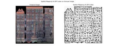
[[File: Spatial mapping lbp.png |400px|thumb|right|an example building façade (left) and its corresponding local binary pattern (LBP) spatial mapping (right)]] | |||
To gain deeper insights into the architectural and typological properties of Venetian facades, we conducted a series of exploratory textural and color analyses, including Local Binary Patterns (LBP) <ref>Ojala, T., Pietikäinen, M., & Mäenpää, T. (2002). Multiresolution grayscale and rotation invariant texture classification with Local Binary Patterns. IEEE Transactions on Pattern Analysis and Machine Intelligence, 24(7), 971–987. doi:10.1109/TPAMI.2002.1017623</ref>, Histogram of Oriented Gradients (HOG)<ref>Dalal, N., & Triggs, B. (2005). Histograms of Oriented Gradients for Human Detection. 2005 IEEE Computer Society Conference on Computer Vision and Pattern Recognition (CVPR’05), Vol. 1, 886–893. doi:10.1109/CVPR.2005.177 | |||
</ref>, and Gabor filters <ref>Gabor, D. (1946). Theory of communication. Journal of the Institution of Electrical Engineers - Part III: Radio and Communication Engineering, 93(26), 429–457. doi:10.1049/ji-3-2.1946.0074 | |||
</ref>. These analysis will potentially provide supportive evidence for model selection, hyperparameters tuning, and error analysis. | |||
=== Local Binary Pattern === | |||
Local Binary Pattern (LBP) encodes how the intensity of each pixel relates to its neighbors, effectively capturing small-scale variations in brightness patterns across the surface. For the facade, this means LBP highlights areas where texture changes—such as the edges around windows, decorative elements, or shifts in building materials—are more pronounced. As a result, LBP maps reveal where the facade’s texture is smooth, where it becomes more intricate, and how these features repeat or vary across different sections of the facades. | |||
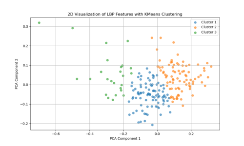
The two-dimensional projection of LBP features via PCA (as shown in the left figure: LBP feature mapping) suggests that the textural characteristics of Venetian facades span a broad and continuous range, rather than forming a few discrete, well-defined clusters. Each point represents the LBP-derived texture pattern of a given image region or facade sample, and their spread across the plot indicates variation in texture complexity, detailing, and material transitions. If there were strong, distinct groupings in this PCA space, it would imply that certain facade types or architectural features share very similar texture signatures. Instead, the relatively diffuse distribution implies that Venetian facades exhibit a wide spectrum of subtle texture variations, with overlapping ranges of structural and decorative elements rather than neatly separable categories. | |||
<gallery mode="packed-hover", heights=200px> | |||
File:lbp_features_kmeans.png |LBP feature mapping | |||
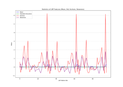
File:Lbp_statistics.png |LBP statistics | |||
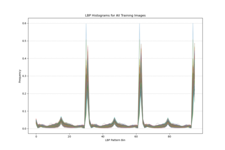
File:Lbp_histograms.png |LBP histogram | |||
</gallery> | |||
The histogram plot (as shown in the right figure: LBP histagram), displaying LBP distributions for all training images, shows pronounced peaks at certain pattern bins rather than a uniform or random spread, indicating that specific local texture patterns are consistently prevalent across the facades. The statistical plot as shown in the middle (mean, standard deviation, kurtosis, skewness) further reveals that these patterns are not normally distributed; some bins have notably high kurtosis and skewness, indicating that certain textures appear more frequently and in a more clustered manner than others. In other words, Venetian facades are characterized by stable, repetitive textural signatures—likely reflecting repeated architectural elements and material arrangements—rather than exhibiting uniformly varied surface textures. | |||
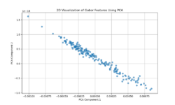
[[File:Gabor_features_pca.png|250px|thumb|right|Gabor Features after PCA(n=2) ]] | |||
=== Gabor Filter === | |||
Gabor filters capture localized frequency and orientation components of an image’s texture. The PCA projection resulting in a near-linear distribution of points suggests that variation in the Gabor feature space is largely dominated by a single principal direction or a narrow set of related factors. This could imply that Venetian facades have a relatively uniform textural pattern, strongly influenced by a consistent orientation or repetitive decorative elements. In other words, the facades’ texture patterns may be comparatively regular and structured, leading to a low-dimensional representation where one main factor (like a dominant orientation or repetitive structural motif) explains most of the variation. | |||
=== Histogram of Oriented Gradients (HOG) === | |||
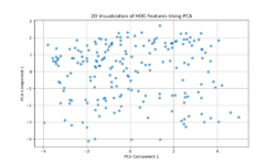
[[File: Hog_features_pca.png |250px|thumb|right|Histogram of Oriented Gradients after PCA(n=2)]] | |||
Histogram of Oriented Gradients (HOG) features capture edge directions and the distribution of local gradients. The more scattered PCA plot indicates that no single dimension dominates the variability as strongly as in the Gabor case. Instead, Venetian facades exhibit a richer diversity of edge and shape information — windows, balconies, ornaments, and varying architectural details produce a more heterogeneous distribution of gradient patterns. This complexity results in a PCA space without a clear linear trend, reflecting more complexity and variety in structural features and contour arrangements. | |||
In Summary | In Summary, Gabor Feature suggest a more uniform, repetitive texture characteristic of Venetian facades, possibly reflecting dominant architectural rhythms or orientation patterns. HOG Features highlight a more diverse set of edge and shape variations, indicating that while texture may be consistent, the facades have numerous structural details and differing configurations that result in a more dispersed feature representation. Together, these indicate that Venetian facades are simultaneously texturally coherent yet architecturally varied in their structural details. | ||
== Methodology == | |||
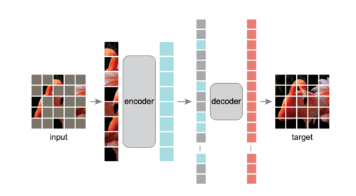
[[File:mae_structure.png|thumb|right|500px|Masked Autoencoder Structure]] | |||
This project is inspired by the paper "Masked Autoencoders Are Scalable Vision Learners" by He et al.<ref>He, K., Chen, X., Xie, S., Li, Y., Dollár, P., & Girshick, R. (2022). Masked Autoencoders Are Scalable Vision Learners. Proceedings of the IEEE/CVF Conference on Computer Vision and Pattern Recognition (CVPR), 16000–16009. https://openaccess.thecvf.com/content/CVPR2022/papers/He_Masked_Autoencoders_Are_Scalable_Vision_Learners_CVPR_2022_paper.pdf</ref>, from Facebook AI Research (FAIR). The Masked Autoencoder splits an image into non-overlapping patches and masks a significant portion (40% to 80%) of them. The remaining visible patches are passed through an encoder, which generates latent representations. A lightweight decoder then reconstructs the entire image, including the masked regions, using these latent features and position embeddings of the masked patches. | |||
The model is trained using a reconstruction loss (e.g., Mean Squared Error) computed only on the masked patches. This ensures the model learns to recover unseen content by leveraging contextual information from the visible patches. The simplicity and efficiency of this approach make MAE highly scalable and effective for pretraining Vision Transformers (ViTs) on large datasets. | |||
By masking a substantial part of the image, MAEs force the model to capture both global structure and local details, enabling it to learn rich, generalizable visual representations. | By masking a substantial part of the image, MAEs force the model to capture both global structure and local details, enabling it to learn rich, generalizable visual representations. | ||
| Line 158: | Line 164: | ||
====Data Preprocessing==== | ====Data Preprocessing==== | ||
Images were resized to a fixed resolution | Images were resized to a fixed resolution of 224x224 and normalized to have pixel values in the range [-1, 1]. The input images were divided into patches of size 16x16, resulting in a grid of 14x14 patches for each image. To improve model generalization, data augmentation techniques were applied during training, including random horizontal flips, slight random rotations, and color jittering (brightness, contrast, and saturation adjustments). These augmentations helped to introduce variability into the small dataset and mitigate overfitting. | ||
We experimented with several image sizes and patch sizes to optimize the model performance. However, we ultimately adopted the same image size (224x224) and patch size (16x16) as the pretrained MAE because they were showing good results and facilitated a direct comparison of results. | |||
==== Model Architecture ==== | |||
The Masked Autoencoder (MAE) consists of an Encoder and a Decoder, designed to reconstruct masked regions of input images. | |||
''' Encoder ''' | |||
The encoder processes visible patches of the image and outputs a latent representation. It is based on a Vision Transformer (ViT) with the following design: | |||
The encoder | |||
Decoder | *12 Transformer layers | ||
The decoder | *Each layer includes Multi-Head Self-Attention (MHSA) with 4 attention heads and a Feed-Forward Network (FFN) with a hidden dimension of 1024. | ||
*Patch embeddings have a dimension of 256. | |||
*Positional embeddings are added to retain spatial information for each patch. | |||
*A CLS token is included to aggregate global information. | |||
The encoder outputs the latent representation of visible patches, which is passed to the decoder. | |||
''' Decoder ''' | |||
The decoder reconstructs the image by processing both the encoded representations of visible patches and learnable masked tokens. It includes: | |||
*6 Transformer layers | |||
*Each layer has Multi-Head Self-Attention (MHSA) with 4 attention heads and a Feed-Forward Network (FFN) with a hidden dimension of 1024. | |||
*A linear projection head maps the decoder output back to pixel values. | |||
*The decoder reconstructs the masked patches and outputs the image in its original resolution. | |||
==== Image Representation ==== | |||
*The input image is divided into patches of size 16x16, creating a grid of 14x14 patches for an image size of 224x224. | |||
*Mask tokens replace the masked regions, and the decoder predicts their pixel values to reconstruct the full image. | |||
By combining this Transformer-based encoder-decoder structure with the masking strategy and positional embeddings, the model effectively learns to reconstruct missing regions in the input images. | |||
====Masking Strategy==== | ====Masking Strategy==== | ||
| Line 177: | Line 205: | ||
====Loss Function==== | ====Loss Function==== | ||
[[File: Loss_picture.png |400px|thumb|right]] | |||
To optimize the model, I used a combination of Masked MSE Loss and Perceptual Loss. The Masked MSE Loss, following the original MAE methodology, is computed only on the masked patches to encourage reconstruction of unseen regions. The Perceptual Loss, derived from a pre-trained VGG19 network, enhances reconstruction quality by focusing on perceptual similarity, also restricted to masked regions, the final loss is a weighted combination. | |||
====Training and Optimization==== | ====Training and Optimization==== | ||
| Line 190: | Line 218: | ||
Performance was evaluated based on reconstruction quality (MSE + perceptual loss) and visual fidelity of reconstructed images. | Performance was evaluated based on reconstruction quality (MSE + perceptual loss) and visual fidelity of reconstructed images. | ||
===Pre- | ---- | ||
===Pre-trained MAE=== | |||
The chosen model is a large MAE-ViT architecture pretrained on ImageNet. This model is configured as follows: | |||
<pre> | |||
def mae_vit_large_patch16_dec512d8b(**kwargs): | |||
model = MaskedAutoencoderViT( | |||
patch_size=16, embed_dim=1024, depth=24, num_heads=16, | |||
decoder_embed_dim=512, decoder_depth=12, decoder_num_heads=16, | |||
mlp_ratio=4, norm_layer=partial(nn.LayerNorm, eps=1e-6), **kwargs) | |||
return model | |||
</pre> | |||
This configuration reflects a ViT-Large backbone with a 16×16 patch size, a high embedding dimension (1024), and a substantial encoder/decoder depth. The original MAE is designed with random patch masking in mind (i.e., a masking ratio of 0.75). This backbone was pretrained on ImageNet and, in the approach described here, is further adapted for facade reconstruction by finetuning certain components. | |||
The experiments discussed here begin by utilizing a specific checkpoint that incorporates an additional Generative Adversarial Network (GAN) loss component. This checkpoint, provided by the Facebook Research team, can be accessed and downloaded from the following link: [https://dl.fbaipublicfiles.com/mae/visualize/mae_visualize_vit_large_ganloss.pth Download checkpoint here] | |||
This enhanced checkpoint has been trained beyond standard MAE objectives, likely giving it a more nuanced understanding of global and local image features. This serves as a strong baseline for finetuning on the facade dataset. | |||
'''Freezing the Encoder and Extending the Decoder:''' | |||
The encoder parameters are frozen, as they contain general pre-learned features from ImageNet. The decoder is then reintroduced and extended by adding more layers to better capture the architectural details of facades. Increasing the decoder depth provides a larger capacity for complex feature transformations and more nuanced reconstructions. A deeper decoder can better capture subtle architectural details and textures that are characteristic of building facades. Thus, these improvements can be attributed to the increased representational power and flexibility of a deeper decoding network. | |||
The model, pretrained on ImageNet, “knows” a wide range of low-level and mid-level features (e.g., edges, textures) common in natural images. It can leverage these features for initial facade reconstruction tasks. The pretrained weights provide a strong initialization, speeding up convergence and improving stability. The model can quickly learn general color and shape distributions relevant to images. The ImageNet backbone does not specialize in architectural patterns. Without fine-tuning, it may overlook domain-specific features (e.g., window shapes, door frames). Thus, while it provides a broad visual language, it lacks a priori understanding of facade-specific semantics and must learn these details through finetuning. | |||
==== Masking and sharpening strategies ==== | |||
'''Random masking:''' | |||
The MAE model uses random masking, where patches are randomly removed and the network learns to reconstruct them. This ensures that the model evenly learns features across the entire image, promoting a more generalized understanding of the scene. Random masking encourages the model to be robust and to learn global structures. By forcing the network to infer missing content from sparse visual cues distributed throughout the image, it ensures that no single area dominates training. This results in the model being better at reconstructing a wide range of features, as opposed to overfitting to a particular region or pattern. | |||
The | |||
To improve reconstruction sharpness and detail fidelity, additional techniques were explored: | |||
<div style="margin-left: 30px;"> | |||
'''Perceptual Loss via VGG:''' | |||
Perceptual loss functions compare high-level feature representations of the output and target images as extracted by a pretrained VGG network. By emphasizing the similarity of feature maps rather than raw pixel differences, the model is encouraged to produce more visually pleasing and structurally coherent reconstructions. This can help maintain repetitive features and stylistic elements characteristic of facades. The main goal is to enhance the quality and realism of the reconstructed images. Perceptual loss promotes the retention of global structural patterns and textures, making the result less blurry and more visually appealing, which is crucial for architectural details. | |||
'''Refinement U-Net:''' | |||
A refinement U-Net is introduced as a post-processing network to improve fine details. This network can: | |||
While NMF-based reconstruction | * Denoise outputs. | ||
* Reduce artifacts introduced by the initial reconstruction. | |||
* Enhance edges and textures. | |||
* Correct color inconsistencies. | |||
This step involves passing the MAE output through a lightweight model that is trained to produce a cleaner, sharper final image. | |||
</div> | |||
'''Block masking - a hybrid approach:''' | |||
While random masking is suitable for training, it does not reflect the actual inference scenario where large, contiguous sections of the facade (e.g., the lower portion corresponding to doors and entrances) might be missing or heavily occluded. The goal is to teach the model to handle such structured absence of data. With this in mind, we would also like to implement a '''biased block masking''' that is biased toward the lower portion of the image. Essentially, we would like to teach the model, who often has the 'head' of the facades (e.g. the top portion, consisting of roofs and upper windows) but no body, how to be able to learn what a 'body' should look like (e.g. the lower details of facades, including doors, balconies, and arches). | |||
When block masking replaces random masking, performance should initially degrade. The model, which has adapted to random patch-level holes, must now handle larger, contiguous missing areas. To mitigate this, a staged approach is recommended: | |||
*'''Warm-Up with Random Masking:''' Train initially with random masking to learn global facade structures. In this way, it will be able to learn and catch low-placed details such as doors and ledges. | |||
*'''Transition to Block Masking:''' Gradually introduce block-based masking, allowing the model to adapt without abruptly losing the benefits of global pattern recognition. | |||
''Why not entirely train with block masking if that is the end goal?'' The model may learn how to handle large missing sections but might fail to develop a robust understanding of global patterns, such as these lower areas we have mentioned. Thus, we motivate training with random masking during a certain number of warmup epochs to avoid this. | |||
---- | |||
=== Non-negative Matrix Factorization === | |||
Non-Negative Matrix Factorization (NMF) has emerged as a powerful tool for dimensionality reduction and feature extraction, particularly suited to applications where data are inherently non-negative. In image processing tasks, NMF can be applied to reconstruct missing regions in incomplete images by decomposing an image into a linear combination of non-negative basis images and corresponding non-negative coefficients. | |||
The incentive to use Nonnegative Matrix Factorization (NMF) for facade image reconstruction is based on several key points: <br> | |||
# NMF provides a relatively simple and easily adjustable model structure. <br> | |||
# NMF can handle outliers and noise more effectively than some complex models. <br> | |||
# The loss function in NMF is fully customizable, which allows for future incorporation of semantic or textural-level loss instead of relying purely on pixel-level errors. <br> | |||
# Compared to methods like Masked Autoencoders (MAE), NMF has significantly fewer hyperparameters, making the model more interpretable. This interpretability is particularly valuable in contexts such as cultural heritage preservation, where clarity in the model’s behavior is crucial. | |||
NMF decomposes a dataset, represented as a large matrix, into two smaller matrices that contain only nonnegative values. The first matrix represents the building blocks or components of the data, while the second matrix specifies how to combine these components to approximate the original data. The number of components is determined by the level of detail required and is chosen based on the specific application. Each component typically captures localized patterns or features, such as windows, edges, or balconies, that are commonly found in facade structures. | |||
The decomposition process aims to minimize the difference between the original data and its approximation based on the two smaller matrices. By ensuring that all values in the matrices are nonnegative, NMF tends to produce parts-based representations. These representations make it easier to interpret which features contribute to the reconstruction of specific areas in the data. | |||
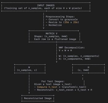
[[File: NMF pipeline.jpg |350px|thumb|right|Non-negative Matrix Factorization Structure and Data Workflow]] | |||
# Input Data (V): | |||
#* Converted to grayscale | |||
#* Resized to a fixed size (256 x 256) | |||
#* Flattened into a single vector. | |||
#* Stacking all these flattened vectors forms a data matrix V with shape (n_samples, img_height * img_width). Here, img_height * img_width = 256 * 256 = 65536 pixels per image. Thus, if we have n_samples images, V is (n_samples x 65536). | |||
# NMF Decomposition (W and H): | |||
#* The NMF model factorizes V into two matrices: W and H. | |||
#* W (of shape (n_samples, n_components)) shows how each of the n_components is combined to construct each of the n_samples images. | |||
#* H (of shape (n_components, img_height * img_width)) encodes the “basis images” or components. Each of the n_components can be thought of as a part or a pattern that, when linearly combined (with non-negative weights), reconstructs the original images. | |||
#* We chose n_components = 60. That means the model tries to explain each image as a combination of 60 “parts” or “features” (stored in rows of H). | |||
# Test Phase (Reconstruction): | |||
#* Loads and preprocesses them similarly. | |||
#* Uses the trained NMF model to get the coefficient matrix H_test (via model.transform) and then reconstructs the images as V_test_reconstructed = H_test × H. | |||
#* The reconstructed images can be combined with the original partial information to generate a final completed image. | |||
While NMF-based reconstruction does not guarantee perfect results, particularly when large parts of the image are missing or the training data is not diverse enough, it often provides semantically meaningful completions. These results are generally better than those achieved through simple pixel-based interpolation. Further improvements could be achieved by integrating complementary techniques, such as texture synthesis or advanced regularization, or by incorporating prior knowledge about architectural structures. | |||
==== Hyperparameter Choice of NMF ==== | ==== Hyperparameter Choice of NMF ==== | ||
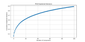
[[File: PCA explained variance.png |300px|thumb|right|PCA explained variance by NMF components]] | |||
# Dimensionality Reduction Insights: <br> | |||
#* PCA Pre-analysis: Before running NMF, apply Principal Component Analysis (PCA) to the training and test images. Analyze the explained variance of PCA components to estimate the intrinsic dimensionality of the data. <br> | |||
#* Reconstruction Saturation: Determine a range of PCA components at which reconstruction quality stops improving significantly. This provides a strong initial guess for the number of components (n_components) in NMF. <br> | |||
# Hyperparameter Decisions for NMF: <br> | |||
#* Number of Components (n_components): Choose a value informed by PCA and by evaluating the reconstruction performance. Strive to capture most of the variance without overfitting. As can be seen from the PCA explained variance, a suitable choice of n_components is 60. <br> | |||
#* Initialization (init): Use nndsvda (Nonnegative Double Singular Value Decomposition with zeroing) for faster convergence and better initial component estimates. <br> | |||
#* Regularization: Consider adding L1 or L2 regularization (via l1_ratio) to promote sparsity or smoothness in the learned components. Decisions on regularization parameters can be guided by cross-validation or domain-specific considerations (e.g., promoting certain architectural features while discouraging noise). However, due to computational time consideration, we only conducted an one-shot experiment to select L1 regularization, which results in smaller reconstruction error. | |||
== Results == | == Results == | ||
=== | ===Custom MAE=== | ||
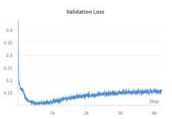
[[File:Val_loss.png|thumb|right|250px|alt=Results at Epoch 350|validation Loss during training, increasing after 300 epochs]] | |||
The results obtained from training our custom MAE were not entirely satisfactory, as the reconstructed images appeared quite blurry and lacked fine-grained details, having difficulty recovering features like windows or edges. The original motivation for training the model from scratch was to have greater flexibility in the model architecture. By building a custom MAE, we aimed to tailor the model's design to the specific challenges of our dataset, such as the unique structure of incomplete facades and the need to experiment with different parameters like masking strategies, patch sizes, and embedding dimensions. This level of customization allowed us to explore architectural decisions that might better align with the characteristics of our data, compared to relying on a pretrained model with fixed design choices but a major limitation in this setup was the size of the dataset, which contained only 650 images of complete facades. Training a deep learning model like an MAE, especially from scratch, requires a much larger dataset to effectively learn meaningful representations. With such a small dataset, the model struggled to generalize, focusing on coarse, low-frequency features such as the overall structure and color distribution, rather than capturing finer details like edges, textures, and patterns. | |||
While the perceptual loss based on VGG19 features did enhance the reconstruction quality, its impact was limited by the small size of the training dataset. The model successfully began to recover higher-level patterns and global structures, such as windows and doors, but struggled to capture fine-grained details due to insufficient training data. During training, the validation loss decreased until approximately epoch 300, after which it began to increase, signaling overfitting. Interestingly, despite the rising loss, the visual quality of the reconstructed images continued to improve up to around epoch 700. This suggests that the model was learning to replicate patterns, such as windows and doors, observed in the training set and applying these learned structures to the facades in the validation set, resulting in more realistic-looking reconstructions. | |||
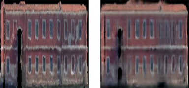
[[File:results_on_the_validation_epoch_350.png|thumb|center|1000px|alt=Results at Epoch 350|At Epoch 350, the model begins to overfit. It captures colors effectively and starts introducing vertical patterns that hint at the formation of windows.]] | |||
[[File:results_on_the_validation_set_epoch_990.png|thumb|center|1000px|alt=Results at Epoch 990|At Epoch 990, despite a higher loss, the model reconstructs features more accurately, showing clearer structures and improved details.]] | |||
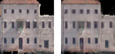
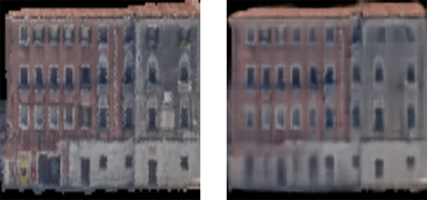
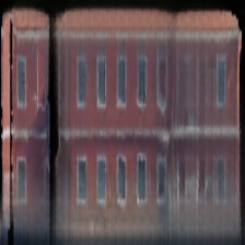
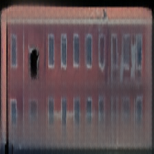
Even though those results seem promising the model demonstrates a notable tendency to reproduce patterns from the training set onto validation facades that share visual similarities. The model memorizes certain features, such as the shape and position of windows or architectural elements, rather than learning generalized representations. In the images below, we observe that parts of the validation reconstructions resemble features seen in the training facades. | |||
<div style="display: flex; justify-content: center; gap: 2%; text-align: center; align-items: center;"> | |||
<div style="width: 45%; text-align: center; max-width: 100%; height: auto;"> | |||
[[File: Facade on the training set 2.png |thumb|center|400px|alt=Training Example|This training example showcases the patterns and structures that the model learns, such as the arrangement of windows and even the small hole in the facade.]] | |||
</div> | |||
<div style="width: 45%; text-align: center; max-width: 100%; height: auto;"> | |||
[[File: Reconstruction_of_a_similar_facade_on_the_validation_set_2.png |thumb|center|400px|alt=Validation Example|In this validation example, the model reproduces the exact same pattern seen in the training image, demonstrating overfitting on certain features.]] | |||
</div> | |||
</div> | |||
This suggests that the model is copying "learned patterns" rather than fully reconstructing unseen details, highlighting the limitations of training with a small dataset. | |||
To overcome these limitations, we opted to use a '''pretrained model''' instead of training from scratch. The pretrained model, fine-tuned on our specific dataset, leveraged learned representations from large-scale training on diverse data, allowing it to generalize much better. By building on the rich, low- and high-level features already embedded in the pretrained network, the fine-tuned model produced significantly sharper and more realistic reconstructions. In the next section, we will present the results obtained using this pretrained model, highlighting its improved performance compared to the custom MAE. | To overcome these limitations, we opted to use a '''pretrained model''' instead of training from scratch. The pretrained model, fine-tuned on our specific dataset, leveraged learned representations from large-scale training on diverse data, allowing it to generalize much better. By building on the rich, low- and high-level features already embedded in the pretrained network, the fine-tuned model produced significantly sharper and more realistic reconstructions. In the next section, we will present the results obtained using this pretrained model, highlighting its improved performance compared to the custom MAE. | ||
== | ---- | ||
===Pre-trained MAE=== | |||
==== Random masking ==== | |||
<gallery mode="packed" heights="120px" style="margin: 40px;"> | |||
File:Facade1_baseline_random.png|Facade 1, with random masking | |||
File:Facade2_baseline_random.png|Facade 2, with random masking | |||
File:Facade3_baseline_random.png|Facade 3, with random masking | |||
</gallery> | |||
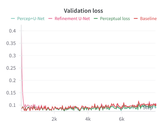
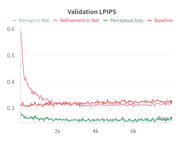
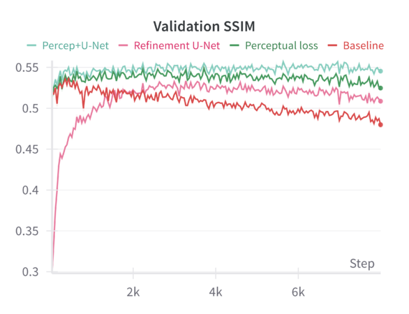
When tested on the filtered dataset of complete facades, the model—finetuned with random masking—generates reconstructions that are coherent but often lack sharp architectural details. Despite training for 200 epochs, the results remain somewhat blurry, and finer architectural features are not faithfully preserved. While random masking helps the model learn global structure, it does not explicitly guide it to emphasize fine details. The model, especially after resizing and losing some aspect ratio information, may rely heavily on learned general features rather than focusing on domain-specific architectural elements. Simply increasing training epochs without additional loss functions or refinement steps does not guarantee sharper reconstructions. The reported '''MSE loss''' on the validation set is '''0.1''', while other metrics such were: '''LPIPS = 0.326''' and '''SSIM = 0.479'''. | |||
We can compare these baseline results across the different sharpening methods in the following graphs: | |||
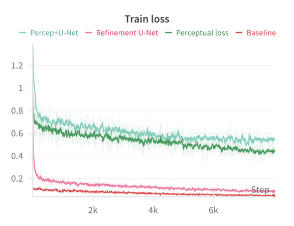
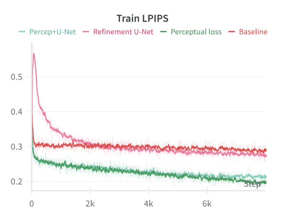
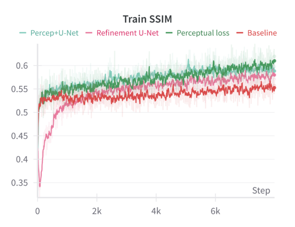
<gallery mode="packed" widths="300px" heights="300px" style="margin: 10px;"> | |||
File:train_loss_comp.png|Train loss (base MSE) | |||
File:train_lpips_comp.png|Train LPIPS | |||
File:final_train_ssim.png|Train SSIM | |||
File:final_val_loss.png|Validation loss (MSE) | |||
File:final_val_lpips.png|Validation LPIPS | |||
File:final_val_ssim.png|Validation SSIM | |||
</gallery> | |||
When finetuning the MAE model on the resized 224×224 facade images using only the standard MAE reconstruction loss (MSE), the model converges smoothly. The validation metrics (including loss, Learned Perceptual Image Patch Similarity—LPIPS, and Structural Similarity Index—SSIM) improve over epochs but do not reach the sharpness or level of structural fidelity necessary to capture subtle architectural details. | |||
Introducing a perceptual loss (derived from pretrained VGG features) naturally raises the training loss values. This increase occurs because perceptual loss measures differences in high-level feature space rather than direct pixel-space discrepancies. While the raw training loss is higher, it decreases following a consistent trend, indicating that the model can still effectively learn under this more stringent criterion. The validation results are notably better: perceptual loss leads to a reduction in LPIPS and improvements in SSIM compared to the baseline. In other words, although the model “struggles” more during training (as reflected in higher loss values), it generalizes better and produces more perceptually pleasing reconstructions. | |||
Applying a refinement U-Net to the MAE output helps restore sharpness, reduce artifacts, and enhance textural details. While the refinement U-Net alone does not always outperform the perceptual loss training by a large margin, it provides consistent gains in visual smoothness and structural integrity. Validation metrics show that refinement alone achieves improvements close to or slightly better than baseline, particularly in SSIM and sometimes LPIPS. | |||
When both perceptual loss and the refinement U-Net are utilized, the results are mildly synergistic. On the validation set, this combination yields the best overall performance across multiple metrics—achieving the lowest loss, the lowest LPIPS values, and the highest SSIM scores. This suggests that the model benefits from both a strong, feature-level training signal (perceptual loss) and a post-hoc enhancement mechanism (refinement U-Net) that restores local details. Although the gain in loss and LPIPS over perceptual loss alone might be slight, the improvement in SSIM is more pronounced, indicating a better structural similarity to ground-truth facades. | |||
=== Hybrid block masking === | |||
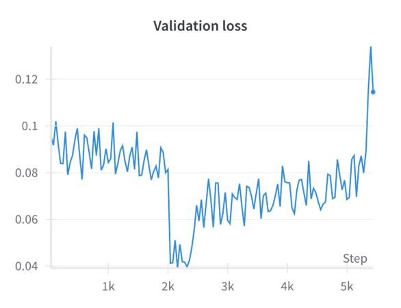
We view the results from a run that started with a 0.4 ratio for block masking and a 0.35 ratio for random masking, and concluded with a 0.6 ratio for block masking and a 0.0 ratio for random masking. | |||
<gallery mode="packed" heights="300px" style="margin: 40px;"> | |||
File:val_loss_hybrid.png|Validation loss with hybrid block masking | |||
File:val_lpips_mixed.png|LPIPS with hybrid block masking | |||
File:val_ssim_mixed.png|SSIM with hybrid block masking | |||
</gallery> | |||
<gallery mode="packed" heights="200px" style="margin: 40px;"> | |||
File:facade1mixed.png|Facade 1, with hybrid block masking | |||
File:facade2mixed.png|Facade 2, with hybrid block masking | |||
File:facade3mixed.png|Facade 3, with hybrid block masking | |||
</gallery> | |||
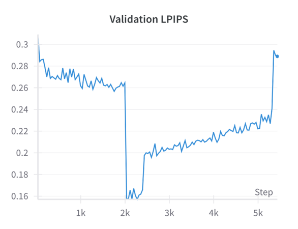
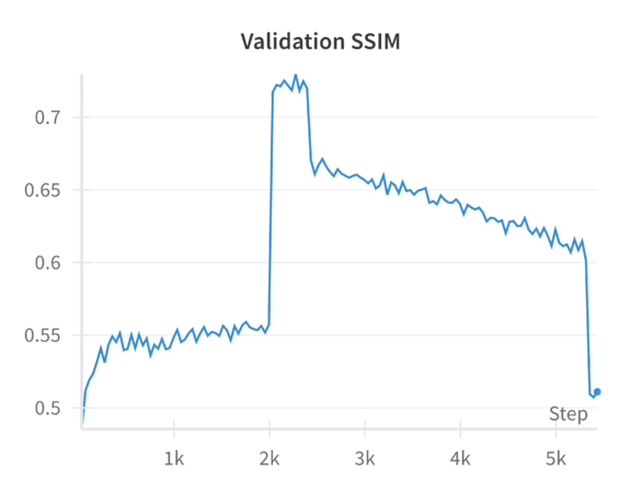
We see that the model is most stable at the beginning with the random masking before gradually improving with the initial combination of block masking and random masking. As the block masking continues to increase across the epochs, we see that performance gradually drops in quality, before more-or-less exploding toward the end. This suggests that this model does not fare well at least in these early stages (200 epochs). | |||
The pretrained MAE model (including the MAE-GAN checkpoint) was originally optimized to handle randomly distributed masked patches. Random masking forces the model to learn a globally consistent representation of the image, as it must infer details from sparse, well-distributed clues. When you suddenly introduce a large portion of block masking—especially concentrated in a single area (e.g., the lower region of the facade)—you fundamentally alter the reconstruction task. Instead of leveraging scattered visual cues that allow the model to piece together the facade from multiple vantage points, the model now faces a more challenging problem: a large, contiguous void. This contiguous gap does not provide the same level of distributed context the model is accustomed to. As a result, the model’s learned representations and attention mechanisms, tuned to handle random patches, may not transfer efficiently. | |||
Random masking is akin to guessing small missing puzzle pieces scattered throughout the image. The model can rely on local and global patterns distributed all over the facade. In contrast, block masking is more like a large, contiguous puzzle piece missing in one region. The model must rely heavily on global architectural semantics and structural regularities to fill this gap. Given that the model was trained primarily under random masking assumptions, it may lack the fine-tuned ability to reconstruct large, context-dependent sections. This is particularly challenging for architectural details that are unevenly distributed and context-specific (e.g., the lower portion of a Venetian facade might include doors, ornate bases, or textural transitions not present in upper areas). | |||
We can view an interesting result that comes from this low-area-biased block masking, which is that: '''everything can be a window'''. | |||
<gallery mode="packed" heights="200px" style="margin: 40px;"> | |||
File:facade1nowindow.png|Facade 1 | |||
File:facade2nowindow.png|Facade 2 | |||
File:facade3nowindow.png|Facade 3 | |||
</gallery> | |||
This is a key result to keep in mind when implementing masking strategies which we foresaw, though maybe the block masking was too aggressive at the beginning causing this to happen. Another thing to consider is that the drastic drop in SSIM and rise in LPIPS indicate that the model’s internal representations have not had enough epochs to adapt to the fundamentally different masking pattern. Progressive block masking partially alleviates the transition by starting with a smaller block ratio and gradually increasing it. However, the number of epochs or the gradual schedule may still be insufficient for the model to “unlearn” its strong bias toward random patch reconstruction and “relearn” a strategy suitable for large contiguous missing areas. | |||
---- | |||
===NMF=== | |||
The reconstructed facades, as illustrated by the provided examples, exhibit several noteworthy characteristics: | |||
* Structural Consistency: The NMF-based approach recovers the general shape and broad architectural features of the buildings depicted. For example, window placements, building outlines, and large-scale contrasts are reasonably reconstructed. This demonstrates that the NMF basis images effectively capture dominant spatial patterns and that these patterns can be recombined to fill missing areas. | |||
* Smoothness of Reconstruction: Due to the nature of NMF’s additive combinations, reconstructions tend to be smooth and free from negative artifacts. This results in visually coherent fills rather than abrupt transitions or unnatural patterns. | |||
* Spatial Averaging Effects: While the global structure is often well approximated, finer details, such as small textural features or subtle contrast differences, are sometimes lost. NMF often produces reconstructions that appear slightly blurred or smoothed, especially in regions with fine-grained details. | |||
* Sensitivity to Initialization and Rank Selection: NMF’s performance is sensitive to the choice of the latent dimensionality (i.e., the rank) and initialization. A suboptimal rank may lead to oversimplified basis images that cannot capture finer nuances, whereas too high a rank could lead to overfitting and less stable reconstructions. | |||
* Limited Contextual Reasoning: Since NMF relies purely on the statistical structure within the image data and does not inherently model higher-level semantics, certain patterns, especially those not well-represented in the known portions of the image, are not reconstructed convincingly. Complex structural features or patterns unique to missing regions may be poorly recovered without additional constraints or priors. | |||
2. | <gallery mode="slideshow"> | ||
File:NMF Inpainting Examples 1.png | |||
File:NMF Inpainting Examples 2.png | |||
</gallery> | |||
When compared to more advanced methods such as MAE, NMF reconstructions generally lag behind in terms of high-frequency detail recovery and semantic consistency. NMF does not exploit spatial correlation beyond low-rank approximations and lacks explicit regularization that encourages edge continuity, object-level coherence, or natural texture synthesis. Nonetheless, NMF remains appealing due to its relative conceptual simplicity, interpretability, and guaranteed non-negativity. | |||
Several promising avenues can enhance the performance of NMF-based image reconstruction, while due to the timeframe we are unable to implement and experiment with them, we document following future improvements here: | |||
* Introducing spatial priors or regularization terms (e.g., total variation regularization or Laplacian smoothing) can help preserve edges and reduce blurring. Such constraints could maintain sharper boundaries and more coherent structural details in the reconstructed image. | |||
* Rather than relying on a fixed set of basis images learned solely from the incomplete image, external databases or a collection of representative images could be used to guide NMF basis selection. Domain-specific dictionaries that capture known structural patterns could improve reconstruction quality. | |||
* Employing a hierarchical NMF framework that decomposes images at multiple scales may recover both global structures and local details. At coarser scales, broad patterns can be learned, while finer scales capture subtle textures and edges, merging these representations for improved fidelity. | |||
* Combining NMF with complementary approaches may offer significant benefits. For instance, one could use NMF to produce an initial coarse reconstruction and then apply a subsequent refinement stage (e.g., a deep learning-based inpainting method) to recover finer details. Such a hybrid method leverages the interpretability and stability of NMF while benefiting from the representational power of more complex models. | |||
* Weighted NMF or robust NMF variants that account for noise and outliers can be adapted to the image reconstruction setting. By explicitly modeling pixel reliability or employing loss functions less sensitive to outliers, the reconstructions may become more accurate and stable. | |||
== Error Analysis: Linking Feature Representations to MAE Reconstruction == | |||
The Gabor features highlight repetitive, uniform texture patterns within the Venetian facades. Often, these facades display recurring motifs such as brick patterns, stone arrangements, or consistent color gradients. The Gabor analysis indicates that the texture frequency and orientation within these facades vary predominantly along a one-dimensional axis, suggesting a strong commonality in their underlying textural structures. As a consequence, Masked Autoencoders (MAEs) can more easily infer missing parts of these uniform textures because their global context and repetitive nature guide the reconstruction. When a portion of a patterned surface—such as an area of uniform masonry—is masked, the MAE can rely on its learned context to fill in the missing pixels accurately, resulting in low reconstruction errors for these texturally consistent regions. | |||
On the other hand, the Histogram of Oriented Gradients (HOG) features capture the distribution of edges, corners, and shapes formed by architectural elements. Venetian facades are adorned with diverse details, including windows, balconies, moldings, and columns, all contributing to a rich variety of edge patterns. The Principal Component Analysis (PCA) of HOG features reveals a more scattered distribution, indicating the absence of a single dominant edge pattern “type.” Instead, there is a broad spectrum of architectural elements with unique, often intricate features. For MAEs, this diversity complicates the prediction of masked areas containing unique details. Unlike repetitive textures, where global context suffices, a distinctive balcony or uncommon decorative element offers few cues that can be extrapolated from surrounding structures. Consequently, the MAE may produce broadly plausible reconstructions but fail to capture subtle intricacies, leading to greater reconstruction errors in these irregularly detailed regions. | |||
Structural regularity and symmetry, as revealed by Local Binary Patterns (LBP), further inform the understanding of how MAEs reconstruct Venetian facades. LBP analysis shows pervasive repeating patterns and symmetrical arrangements that the MAE can effectively reproduce. It excels at preserving overarching architectural structures—such as aligned windows and sequences of arches—reflecting the MAE’s strength in capturing large-scale geometric coherence. However, LBP also indicates regions where surfaces transition from smooth to intricate textures. These finely textured areas pose a challenge for the MAE, which tends to simplify complex local details while remaining focused on the broader structure. As a result, while smooth surfaces are faithfully reconstructed due to their low variance, areas rich in detail appear blurred. | |||
This interplay between global form and local nuance is encapsulated by the distinctions that LBP draws between smooth and heavily ornamented areas. Smooth regions, easily modeled and predicted, are reliably restored by the MAE. In contrast, heavily ornamented zones, replete with delicate patterns and subtle variations, are more difficult to recreate with full fidelity. The hierarchical architectural features highlighted by LBP provide further insight: the MAE successfully handles certain levels of architectural complexity—such as maintaining facade outlines and window placements—because these patterns are part of a larger, cohesive structure that the MAE can learn from global context. Yet it struggles with finer ornamental elements that lack such hierarchical repetition. By understanding the hierarchical nature of Venetian facades, it becomes evident why global forms are preserved while delicate details inevitably fade in the MAE’s reconstructions. | |||
== Conclusion == | == Conclusion == | ||
== | The experiments conducted with the '''Masked Autoencoder''' revealed important insights into the reconstruction of facade images. Initially, we trained a '''MAE from scratch''' with block-based masking to better simulate occlusions in partial facades. While this approach allowed flexibility in architectural choices, the results were constrained by the limited dataset size, leading to blurry reconstructions and a lack of fine-grained details. | ||
To address this, we fine-tuned a '''pretrained MAE''' that was originally trained with random masking. Fine-tuning significantly improved reconstruction quality, particularly when using random masking, as the pretrained model's learned representations aligned with this masking strategy. However, the pretrained model struggled to perform well under '''block-based masking''', likely because its pretraining did not include this specific occlusion pattern. This highlights the importance of aligning pretraining strategies with downstream tasks. | |||
=== Future Directions === | |||
==== Pre-trained MAE ==== | |||
Given the good performance of the random masking on the complete facades and the subpar performance of the hybrid masking, we have the following suggestions for improvement: | |||
1. Longer or Two-Phase Training: | |||
Instead of expecting the model to adapt to progressive block masking within the same training run and over a limited number of epochs, consider a two-stage approach: | |||
* Stage 1 (Random Masking): Train or finetune with random masking to establish strong global feature representations. | |||
* Stage 2 (Block Masking): After convergence at Stage 1, continue training from that checkpoint but now introduce block masking more gradually and over many more epochs. This gives the model ample time to adapt its representations and internal heuristics specifically for large contiguous missing regions. | |||
2. Intermediate Masking Strategies: | |||
Before moving fully into large contiguous blocks, consider the following strategies: | |||
* Clumping?: Start by grouping a few masked patches to form slightly bigger clusters, but not full large blocks. Over time, merge these clusters into even larger blocks. This gentle transition might help the model gradually learn to infer larger structures. | |||
*Multi-Scale Masking: Introduce block masking at various scales (small blocks to medium, then large), allowing the model to progressively learn the inpainting task at multiple levels of granularity. | |||
3. Architecture and Loss Modifications: | |||
Since inpainting large regions is a complex task, we can consider architectural modifications or additional loss terms: | |||
* Additional Perceptual and Adversarial Losses: Continue using perceptual loss, and possibly consider a more specific adversarial setup for inpainting (such as a patch-based discriminator focusing on the inpainted region). This was attempted by trying to implement a GAN loss, but not much time was dedicated to really implementing it. | |||
4. Leveraging EDA Insights: | |||
The exploratory analyses (LBP, Gabor, HOG) revealed complex, continuous variations in texture and gradient distributions. You could use these insights as additional priors: | |||
* Region-Specific Conditioning: If the lower portion of Venetian facades has distinctive features, consider providing the model with positional embeddings or metadata that indicate which part of the building it is reconstructing. This extra information can help the model guess architectural elements more accurately. | |||
5. Extended Training With Refinement Steps: | |||
If refinement U-Nets helped after random masking, they may be even more essential when dealing with block masking. First, let the MAE produce a coarse inpainting result. Then, apply a refinement U-Net that has been trained specifically to handle large missing areas. Over time, this two-step process might produce better results than trying to solve the entire problem with one architecture and loss function. | |||
---- | |||
==== Other considerations ==== | |||
[[File: missing_area.png |400px|thumb|right|The "true" areas that need to be inpainted identified by Ramer–Douglas–Peucker (RDP) ratio and y-coordinate]] | |||
[[File: textural_material.png|400px|thumb|right|Different feature representations of a Venetian building facade. The top-left image shows the distribution of Local Binary Patterns (LBP), highlighting textural microstructures. The top-right image presents Gabor features (mean response), capturing oriented textures and edges. The bottom-left image illustrates a material clustering map, distinguishing regions with similar surface characteristics. The bottom-right image displays the building in the L-channel of the LAB color space, emphasizing luminance variations and shading.]] | |||
Extending the pipeline to include a '''detection model''' that identifies and localizes the missing or occluded parts of the facade. Specifically: | |||
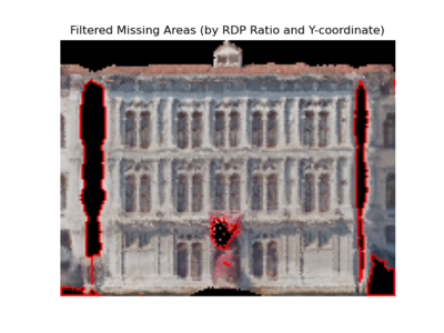
1) Instead of randomly masking square patches, as is common in standard Masked Autoencoder (MAE) pipelines, it is more effective to directly '''identify the specific regions that genuinely require inpainting'''. This approach ensures that the MAE focuses on reconstructing truly missing parts of the data, rather than inadvertently altering intact sections of the image. To achieve this, one can analyze the geometric properties of contours that outline potential missing areas and apply contour simplification algorithms, such as the Ramer–Douglas–Peucker (RDP) algorithm <ref> Ramer, U. (1972). An iterative procedure for the polygonal approximation of plane curves. Computer Graphics and Image Processing, 1(3), 244–256. doi:10.1016/S0146-664X(72)80017-0</ref><ref>Douglas, D. H., & Peucker, T. K. (1973). Algorithms for the Reduction of the Number of Points Required to Represent a Digitized Line or its Caricature. Cartographica: The International Journal for Geographic Information and Geovisualization, 10(2), 112–122. doi:10.3138/FM57-6770-U75U-7727</ref>. | |||
The RDP algorithm approximates complex contours with fewer points while retaining their essential shape. By examining the resulting simplified contours, one can distinguish between regions that are genuinely missing due to data loss and those that merely appear missing because they are obscured by other objects (such as overlapping facades) or cast shadows. Regular, smoothly simplified contours—often approximating geometric shapes like rectangles—are more likely to represent occlusions or overshadowed areas that do not require inpainting. In contrast, regions with irregular, non-uniform contours that remain complex even after RDP simplification are more plausibly true missing areas caused by experimental constraints, sensor malfunctions, or environmental factors like foliage interference. Identifying such irregular contours with RDP enables a targeted inpainting strategy that improves the quality and relevance of the reconstructed data (as in an example shown on the right). | |||
2) By directly '''integrating more feature representations''' (as in figure shown on the right) into the Masked Autoencoder (MAE) pipeline, one can provide the model with richer priors that guide the inpainting process more effectively. For instance, instead of relying solely on raw RGB inputs, additional channels derived from Local Binary Patterns (LBP) and Gabor features can be concatenated or fused into the MAE’s encoder input. This way, the model receives explicit signals about local texture directionality, micro-structure repetitions, and edge distributions. Likewise, the LAB luminance channel offers cues on shading and brightness gradients, while material clustering maps highlight spatially coherent regions, allowing the model to group visually similar areas and maintain consistent texture and color properties within each masked patch. This multi-channel input strategy ensures the latent representations in the MAE capture both low-level textures and higher-level structural semantics, making it easier for the decoder to reconstruct missing segments accurately. | |||
From an architectural perspective, the MAE can be adapted to process these features through parallel branches or specialized attention layers that learn to weight and blend the different modalities. By incorporating loss functions that penalize discrepancies not only in pixel space but also in the feature space (e.g., ensuring that reconstructed textures have similar LBP/Gabor statistics), the training process encourages the network to leverage these additional inputs more effectively. Furthermore, the inclusion of material segmentation maps as priors for masking strategies (e.g., preferring to mask regions that are contextually distinct in material composition) can enhance the MAE’s ability to learn robust completion patterns. Overall, these technical adaptations allow the MAE to move beyond naive pixel-level patch prediction towards a more context-aware, structure-preserving, and material-consistent inpainting approach. | |||
3) '''Partial Facades''': Once the model has successfully identified genuinely missing or occluded areas within the facade imagery, the trained MAE can be deployed to reconstruct these regions. Rather than relying solely on synthetic, randomly placed patches during training, '''employing an MAE on segments explicitly identified as missing''' allows the model to engage with more contextually relevant structures. For instance, if the detection model isolates irregularly shaped gaps—likely due to data loss or actual occlusions—the MAE can focus its latent representations on these specific anomalies. By doing so, the inpainting process moves beyond simple pattern replication, employing the learned embeddings to infer plausible architectural elements, color gradients, and textures that align with the global aesthetic and structural semantics of Venetian facades. Fine-tuning the MAE on partial facade datasets, which contain a range of occlusion levels and missing detail intensities, further refines the model’s ability to handle intricate architectural patterns. This additional training step encourages adaptability and robustness, enabling the MAE to produce realistic reconstructions even under challenging conditions, such as when large portions of the image remain unseen or feature subtle architectural motifs requiring careful inference. | |||
By addressing these future directions, the MAE can be effectively utilized for '''practical inpainting tasks''', enabling the restoration of incomplete facades while preserving architectural coherence. This would be particularly valuable for urban restoration projects, virtual reconstructions, and similar real-world applications. | |||
== References == | == References == | ||
Latest revision as of 22:59, 18 December 2024
Introduction
Motivation
The reconstruction of Venetian building facades is an interdisciplinary challenge, combining computer science, computer vision, the humanities, and architectural studies. Machine Learning (ML) and Deep Learning (DL) techniques offer a powerful solution to fill gaps in 2D facade data for historical preservation and visualization.
Facades vary significantly in structure, size, and completeness, making classical interpolation and rule-based methods inefficient. The Masked Autoencoder (MAE), a Transformer-based model, excels at learning patterns from large datasets and efficiently reconstructing missing regions. With its high masking ratio of 0.75, the MAE can learn robust representations while reconstructing large portions of missing data, making it seem ideal for processing the thousands of facades available to us in our dataset. The MAE captures both high-level structures (e.g., windows, arches) and fine details (e.g., textures, edges) by learning hierarchical features. Thus, it appears ideal for addressing the challenge of maintaining the architectural integrity of reconstructions, preserving stylistic elements crucial for historical analysis.
Venetian facades are valuable artifacts of cultural heritage. The MAE's ability to reconstruct deteriorated or incomplete structures supports digital preservation, enabling scholars and the public to analyze and visualize architectural history. By automating the reconstruction process, the MAE ensures scalable and accurate preservation of these historical assets. The Masked Autoencoder’s adaptability, scalability, and masking ratio of 0.75 make it uniquely suited to this reconstruction project. It efficiently handles large datasets, captures architectural details, and supports the digital preservation of Venice's rich cultural heritage.
Deliverables
Link to the Github respository : https://github.com/yasminek-g/Facade-Autoencoder
Project Timeline & Milestones
| Timeframe | Goals | Tasks |
|---|---|---|
| Week 4 |
|
|
| Week 5 |
|
|
| Week 6 |
|
|
| Week 7 |
|
|
| Week 8 |
|
|
| Week 9 |
|
|
| Week 10 |
|
|
| Week 11 |
|
|
| Week 12 |
|
|
| Week 13 |
|
|
| Week 14 |
|
|
Dataset
Description
The dataset comprises 14,148 building facades extracted from a GeoPandas file. Each facade is represented not by full raw images, but by compressed NumPy arrays containing pointcloud coordinates and corresponding RGB color values. These arrays are discretized into 0.2×0.2 bins, ensuring all images share a uniform “resolution” in terms of bin size. Although different facades vary substantially in physical dimensions, the binning ensures computational uniformity.
Statistical Analysis of Facade Dimensions:
- Mean dimensions: (78.10, 94.78)
- Median dimensions: (78, 79)
- 10th Percentile: (54, 35)
- 90th Percentile: (102, 172)
- 95th Percentile: (110, 214)
While the largest facades remain manageable within typical image model input sizes (e.g., 110×214), the wide variation in size presents a challenge for standard machine learning models, which generally require fixed input dimensions.
Preprocessing strategies
One initial idea was to preserve each facade’s aspect ratio and pad images to standard dimensions. However, padding introduces non-informative regions (often represented as black pixels) that can distort training. If such padding is considered “informative,” the model may learn to reconstruct black areas instead of meaningful details. Ignoring these regions in the loss function similarly leads to losing valuable detail along facade edges. This ultimately prompted the decision to simply resize each image to 224×224 pixels, which aligns with the pretrained MAE model’s requirements. Since all facades are smaller than or approximately equal to the target size, this resizing generally involves upsampling. Nearest-neighbor interpolation is used to preserve color values faithfully without introducing interpolated data that could confuse the reconstruction process.
Exploratory Data Analysis
To gain deeper insights into the architectural and typological properties of Venetian facades, we conducted a series of exploratory textural and color analyses, including Local Binary Patterns (LBP) [1], Histogram of Oriented Gradients (HOG)[2], and Gabor filters [3]. These analysis will potentially provide supportive evidence for model selection, hyperparameters tuning, and error analysis.
Local Binary Pattern
Local Binary Pattern (LBP) encodes how the intensity of each pixel relates to its neighbors, effectively capturing small-scale variations in brightness patterns across the surface. For the facade, this means LBP highlights areas where texture changes—such as the edges around windows, decorative elements, or shifts in building materials—are more pronounced. As a result, LBP maps reveal where the facade’s texture is smooth, where it becomes more intricate, and how these features repeat or vary across different sections of the facades.
The two-dimensional projection of LBP features via PCA (as shown in the left figure: LBP feature mapping) suggests that the textural characteristics of Venetian facades span a broad and continuous range, rather than forming a few discrete, well-defined clusters. Each point represents the LBP-derived texture pattern of a given image region or facade sample, and their spread across the plot indicates variation in texture complexity, detailing, and material transitions. If there were strong, distinct groupings in this PCA space, it would imply that certain facade types or architectural features share very similar texture signatures. Instead, the relatively diffuse distribution implies that Venetian facades exhibit a wide spectrum of subtle texture variations, with overlapping ranges of structural and decorative elements rather than neatly separable categories.
The histogram plot (as shown in the right figure: LBP histagram), displaying LBP distributions for all training images, shows pronounced peaks at certain pattern bins rather than a uniform or random spread, indicating that specific local texture patterns are consistently prevalent across the facades. The statistical plot as shown in the middle (mean, standard deviation, kurtosis, skewness) further reveals that these patterns are not normally distributed; some bins have notably high kurtosis and skewness, indicating that certain textures appear more frequently and in a more clustered manner than others. In other words, Venetian facades are characterized by stable, repetitive textural signatures—likely reflecting repeated architectural elements and material arrangements—rather than exhibiting uniformly varied surface textures.
Gabor Filter
Gabor filters capture localized frequency and orientation components of an image’s texture. The PCA projection resulting in a near-linear distribution of points suggests that variation in the Gabor feature space is largely dominated by a single principal direction or a narrow set of related factors. This could imply that Venetian facades have a relatively uniform textural pattern, strongly influenced by a consistent orientation or repetitive decorative elements. In other words, the facades’ texture patterns may be comparatively regular and structured, leading to a low-dimensional representation where one main factor (like a dominant orientation or repetitive structural motif) explains most of the variation.
Histogram of Oriented Gradients (HOG)
Histogram of Oriented Gradients (HOG) features capture edge directions and the distribution of local gradients. The more scattered PCA plot indicates that no single dimension dominates the variability as strongly as in the Gabor case. Instead, Venetian facades exhibit a richer diversity of edge and shape information — windows, balconies, ornaments, and varying architectural details produce a more heterogeneous distribution of gradient patterns. This complexity results in a PCA space without a clear linear trend, reflecting more complexity and variety in structural features and contour arrangements.
In Summary, Gabor Feature suggest a more uniform, repetitive texture characteristic of Venetian facades, possibly reflecting dominant architectural rhythms or orientation patterns. HOG Features highlight a more diverse set of edge and shape variations, indicating that while texture may be consistent, the facades have numerous structural details and differing configurations that result in a more dispersed feature representation. Together, these indicate that Venetian facades are simultaneously texturally coherent yet architecturally varied in their structural details.
Methodology
This project is inspired by the paper "Masked Autoencoders Are Scalable Vision Learners" by He et al.[4], from Facebook AI Research (FAIR). The Masked Autoencoder splits an image into non-overlapping patches and masks a significant portion (40% to 80%) of them. The remaining visible patches are passed through an encoder, which generates latent representations. A lightweight decoder then reconstructs the entire image, including the masked regions, using these latent features and position embeddings of the masked patches.
The model is trained using a reconstruction loss (e.g., Mean Squared Error) computed only on the masked patches. This ensures the model learns to recover unseen content by leveraging contextual information from the visible patches. The simplicity and efficiency of this approach make MAE highly scalable and effective for pretraining Vision Transformers (ViTs) on large datasets.
By masking a substantial part of the image, MAEs force the model to capture both global structure and local details, enabling it to learn rich, generalizable visual representations.
For this project, two types of MAEs were implemented:
1) Custom MAE: Trained from scratch, allowing flexibility in input size, masking strategies, and hyperparameters.
2) Pretrained MAE: Leveraged a pretrained MAE, which was finetuned for our specific task.
Custom MAE
Data Preprocessing
Images were resized to a fixed resolution of 224x224 and normalized to have pixel values in the range [-1, 1]. The input images were divided into patches of size 16x16, resulting in a grid of 14x14 patches for each image. To improve model generalization, data augmentation techniques were applied during training, including random horizontal flips, slight random rotations, and color jittering (brightness, contrast, and saturation adjustments). These augmentations helped to introduce variability into the small dataset and mitigate overfitting.
We experimented with several image sizes and patch sizes to optimize the model performance. However, we ultimately adopted the same image size (224x224) and patch size (16x16) as the pretrained MAE because they were showing good results and facilitated a direct comparison of results.
Model Architecture
The Masked Autoencoder (MAE) consists of an Encoder and a Decoder, designed to reconstruct masked regions of input images.
Encoder
The encoder processes visible patches of the image and outputs a latent representation. It is based on a Vision Transformer (ViT) with the following design:
- 12 Transformer layers
- Each layer includes Multi-Head Self-Attention (MHSA) with 4 attention heads and a Feed-Forward Network (FFN) with a hidden dimension of 1024.
- Patch embeddings have a dimension of 256.
- Positional embeddings are added to retain spatial information for each patch.
- A CLS token is included to aggregate global information.
The encoder outputs the latent representation of visible patches, which is passed to the decoder.
Decoder The decoder reconstructs the image by processing both the encoded representations of visible patches and learnable masked tokens. It includes:
- 6 Transformer layers
- Each layer has Multi-Head Self-Attention (MHSA) with 4 attention heads and a Feed-Forward Network (FFN) with a hidden dimension of 1024.
- A linear projection head maps the decoder output back to pixel values.
- The decoder reconstructs the masked patches and outputs the image in its original resolution.
Image Representation
- The input image is divided into patches of size 16x16, creating a grid of 14x14 patches for an image size of 224x224.
- Mask tokens replace the masked regions, and the decoder predicts their pixel values to reconstruct the full image.
By combining this Transformer-based encoder-decoder structure with the masking strategy and positional embeddings, the model effectively learns to reconstruct missing regions in the input images.
Masking Strategy
A contiguous block of patches is masked to simulate occlusion, which more accurately represents the incomplete facades in our data compared to a random masking strategy. A masking ratio of 50% was applied, meaning half of the patches in each image were masked during training.
Loss Function
To optimize the model, I used a combination of Masked MSE Loss and Perceptual Loss. The Masked MSE Loss, following the original MAE methodology, is computed only on the masked patches to encourage reconstruction of unseen regions. The Perceptual Loss, derived from a pre-trained VGG19 network, enhances reconstruction quality by focusing on perceptual similarity, also restricted to masked regions, the final loss is a weighted combination.
Training and Optimization
The model was trained using the AdamW optimizer, with a learning rate scaled based on batch size and a cosine decay scheduler for gradual reduction of learning rates. A warm-up phase was incorporated to stabilize training during the initial epochs.
Evaluation Metrics
Performance was evaluated based on reconstruction quality (MSE + perceptual loss) and visual fidelity of reconstructed images.
Pre-trained MAE
The chosen model is a large MAE-ViT architecture pretrained on ImageNet. This model is configured as follows:
def mae_vit_large_patch16_dec512d8b(**kwargs):
    model = MaskedAutoencoderViT(
        patch_size=16, embed_dim=1024, depth=24, num_heads=16,
        decoder_embed_dim=512, decoder_depth=12, decoder_num_heads=16,
        mlp_ratio=4, norm_layer=partial(nn.LayerNorm, eps=1e-6), **kwargs)
    return model
This configuration reflects a ViT-Large backbone with a 16×16 patch size, a high embedding dimension (1024), and a substantial encoder/decoder depth. The original MAE is designed with random patch masking in mind (i.e., a masking ratio of 0.75). This backbone was pretrained on ImageNet and, in the approach described here, is further adapted for facade reconstruction by finetuning certain components.
The experiments discussed here begin by utilizing a specific checkpoint that incorporates an additional Generative Adversarial Network (GAN) loss component. This checkpoint, provided by the Facebook Research team, can be accessed and downloaded from the following link: Download checkpoint here
This enhanced checkpoint has been trained beyond standard MAE objectives, likely giving it a more nuanced understanding of global and local image features. This serves as a strong baseline for finetuning on the facade dataset.
Freezing the Encoder and Extending the Decoder:
The encoder parameters are frozen, as they contain general pre-learned features from ImageNet. The decoder is then reintroduced and extended by adding more layers to better capture the architectural details of facades. Increasing the decoder depth provides a larger capacity for complex feature transformations and more nuanced reconstructions. A deeper decoder can better capture subtle architectural details and textures that are characteristic of building facades. Thus, these improvements can be attributed to the increased representational power and flexibility of a deeper decoding network.
The model, pretrained on ImageNet, “knows” a wide range of low-level and mid-level features (e.g., edges, textures) common in natural images. It can leverage these features for initial facade reconstruction tasks. The pretrained weights provide a strong initialization, speeding up convergence and improving stability. The model can quickly learn general color and shape distributions relevant to images. The ImageNet backbone does not specialize in architectural patterns. Without fine-tuning, it may overlook domain-specific features (e.g., window shapes, door frames). Thus, while it provides a broad visual language, it lacks a priori understanding of facade-specific semantics and must learn these details through finetuning.
Masking and sharpening strategies
Random masking:
The MAE model uses random masking, where patches are randomly removed and the network learns to reconstruct them. This ensures that the model evenly learns features across the entire image, promoting a more generalized understanding of the scene. Random masking encourages the model to be robust and to learn global structures. By forcing the network to infer missing content from sparse visual cues distributed throughout the image, it ensures that no single area dominates training. This results in the model being better at reconstructing a wide range of features, as opposed to overfitting to a particular region or pattern.
To improve reconstruction sharpness and detail fidelity, additional techniques were explored:
Perceptual Loss via VGG:
Perceptual loss functions compare high-level feature representations of the output and target images as extracted by a pretrained VGG network. By emphasizing the similarity of feature maps rather than raw pixel differences, the model is encouraged to produce more visually pleasing and structurally coherent reconstructions. This can help maintain repetitive features and stylistic elements characteristic of facades. The main goal is to enhance the quality and realism of the reconstructed images. Perceptual loss promotes the retention of global structural patterns and textures, making the result less blurry and more visually appealing, which is crucial for architectural details.
Refinement U-Net:
A refinement U-Net is introduced as a post-processing network to improve fine details. This network can:
- Denoise outputs.
- Reduce artifacts introduced by the initial reconstruction.
- Enhance edges and textures.
- Correct color inconsistencies.
This step involves passing the MAE output through a lightweight model that is trained to produce a cleaner, sharper final image.
Block masking - a hybrid approach:
While random masking is suitable for training, it does not reflect the actual inference scenario where large, contiguous sections of the facade (e.g., the lower portion corresponding to doors and entrances) might be missing or heavily occluded. The goal is to teach the model to handle such structured absence of data. With this in mind, we would also like to implement a biased block masking that is biased toward the lower portion of the image. Essentially, we would like to teach the model, who often has the 'head' of the facades (e.g. the top portion, consisting of roofs and upper windows) but no body, how to be able to learn what a 'body' should look like (e.g. the lower details of facades, including doors, balconies, and arches).
When block masking replaces random masking, performance should initially degrade. The model, which has adapted to random patch-level holes, must now handle larger, contiguous missing areas. To mitigate this, a staged approach is recommended:
- Warm-Up with Random Masking: Train initially with random masking to learn global facade structures. In this way, it will be able to learn and catch low-placed details such as doors and ledges.
- Transition to Block Masking: Gradually introduce block-based masking, allowing the model to adapt without abruptly losing the benefits of global pattern recognition.
Why not entirely train with block masking if that is the end goal? The model may learn how to handle large missing sections but might fail to develop a robust understanding of global patterns, such as these lower areas we have mentioned. Thus, we motivate training with random masking during a certain number of warmup epochs to avoid this.
Non-negative Matrix Factorization
Non-Negative Matrix Factorization (NMF) has emerged as a powerful tool for dimensionality reduction and feature extraction, particularly suited to applications where data are inherently non-negative. In image processing tasks, NMF can be applied to reconstruct missing regions in incomplete images by decomposing an image into a linear combination of non-negative basis images and corresponding non-negative coefficients.
The incentive to use Nonnegative Matrix Factorization (NMF) for facade image reconstruction is based on several key points:
- NMF provides a relatively simple and easily adjustable model structure.
- NMF can handle outliers and noise more effectively than some complex models.
- The loss function in NMF is fully customizable, which allows for future incorporation of semantic or textural-level loss instead of relying purely on pixel-level errors.
- Compared to methods like Masked Autoencoders (MAE), NMF has significantly fewer hyperparameters, making the model more interpretable. This interpretability is particularly valuable in contexts such as cultural heritage preservation, where clarity in the model’s behavior is crucial.
NMF decomposes a dataset, represented as a large matrix, into two smaller matrices that contain only nonnegative values. The first matrix represents the building blocks or components of the data, while the second matrix specifies how to combine these components to approximate the original data. The number of components is determined by the level of detail required and is chosen based on the specific application. Each component typically captures localized patterns or features, such as windows, edges, or balconies, that are commonly found in facade structures.
The decomposition process aims to minimize the difference between the original data and its approximation based on the two smaller matrices. By ensuring that all values in the matrices are nonnegative, NMF tends to produce parts-based representations. These representations make it easier to interpret which features contribute to the reconstruction of specific areas in the data.
- Input Data (V):
- Converted to grayscale
- Resized to a fixed size (256 x 256)
- Flattened into a single vector.
- Stacking all these flattened vectors forms a data matrix V with shape (n_samples, img_height * img_width). Here, img_height * img_width = 256 * 256 = 65536 pixels per image. Thus, if we have n_samples images, V is (n_samples x 65536).
- NMF Decomposition (W and H):
- The NMF model factorizes V into two matrices: W and H.
- W (of shape (n_samples, n_components)) shows how each of the n_components is combined to construct each of the n_samples images.
- H (of shape (n_components, img_height * img_width)) encodes the “basis images” or components. Each of the n_components can be thought of as a part or a pattern that, when linearly combined (with non-negative weights), reconstructs the original images.
- We chose n_components = 60. That means the model tries to explain each image as a combination of 60 “parts” or “features” (stored in rows of H).
- Test Phase (Reconstruction):
- Loads and preprocesses them similarly.
- Uses the trained NMF model to get the coefficient matrix H_test (via model.transform) and then reconstructs the images as V_test_reconstructed = H_test × H.
- The reconstructed images can be combined with the original partial information to generate a final completed image.
While NMF-based reconstruction does not guarantee perfect results, particularly when large parts of the image are missing or the training data is not diverse enough, it often provides semantically meaningful completions. These results are generally better than those achieved through simple pixel-based interpolation. Further improvements could be achieved by integrating complementary techniques, such as texture synthesis or advanced regularization, or by incorporating prior knowledge about architectural structures.
Hyperparameter Choice of NMF
- Dimensionality Reduction Insights:
- PCA Pre-analysis: Before running NMF, apply Principal Component Analysis (PCA) to the training and test images. Analyze the explained variance of PCA components to estimate the intrinsic dimensionality of the data.
- Reconstruction Saturation: Determine a range of PCA components at which reconstruction quality stops improving significantly. This provides a strong initial guess for the number of components (n_components) in NMF.
- PCA Pre-analysis: Before running NMF, apply Principal Component Analysis (PCA) to the training and test images. Analyze the explained variance of PCA components to estimate the intrinsic dimensionality of the data.
- Hyperparameter Decisions for NMF:
- Number of Components (n_components): Choose a value informed by PCA and by evaluating the reconstruction performance. Strive to capture most of the variance without overfitting. As can be seen from the PCA explained variance, a suitable choice of n_components is 60.
- Initialization (init): Use nndsvda (Nonnegative Double Singular Value Decomposition with zeroing) for faster convergence and better initial component estimates.
- Regularization: Consider adding L1 or L2 regularization (via l1_ratio) to promote sparsity or smoothness in the learned components. Decisions on regularization parameters can be guided by cross-validation or domain-specific considerations (e.g., promoting certain architectural features while discouraging noise). However, due to computational time consideration, we only conducted an one-shot experiment to select L1 regularization, which results in smaller reconstruction error.
- Number of Components (n_components): Choose a value informed by PCA and by evaluating the reconstruction performance. Strive to capture most of the variance without overfitting. As can be seen from the PCA explained variance, a suitable choice of n_components is 60.
Results
Custom MAE
The results obtained from training our custom MAE were not entirely satisfactory, as the reconstructed images appeared quite blurry and lacked fine-grained details, having difficulty recovering features like windows or edges. The original motivation for training the model from scratch was to have greater flexibility in the model architecture. By building a custom MAE, we aimed to tailor the model's design to the specific challenges of our dataset, such as the unique structure of incomplete facades and the need to experiment with different parameters like masking strategies, patch sizes, and embedding dimensions. This level of customization allowed us to explore architectural decisions that might better align with the characteristics of our data, compared to relying on a pretrained model with fixed design choices but a major limitation in this setup was the size of the dataset, which contained only 650 images of complete facades. Training a deep learning model like an MAE, especially from scratch, requires a much larger dataset to effectively learn meaningful representations. With such a small dataset, the model struggled to generalize, focusing on coarse, low-frequency features such as the overall structure and color distribution, rather than capturing finer details like edges, textures, and patterns.
While the perceptual loss based on VGG19 features did enhance the reconstruction quality, its impact was limited by the small size of the training dataset. The model successfully began to recover higher-level patterns and global structures, such as windows and doors, but struggled to capture fine-grained details due to insufficient training data. During training, the validation loss decreased until approximately epoch 300, after which it began to increase, signaling overfitting. Interestingly, despite the rising loss, the visual quality of the reconstructed images continued to improve up to around epoch 700. This suggests that the model was learning to replicate patterns, such as windows and doors, observed in the training set and applying these learned structures to the facades in the validation set, resulting in more realistic-looking reconstructions.
Even though those results seem promising the model demonstrates a notable tendency to reproduce patterns from the training set onto validation facades that share visual similarities. The model memorizes certain features, such as the shape and position of windows or architectural elements, rather than learning generalized representations. In the images below, we observe that parts of the validation reconstructions resemble features seen in the training facades.
This suggests that the model is copying "learned patterns" rather than fully reconstructing unseen details, highlighting the limitations of training with a small dataset.
To overcome these limitations, we opted to use a pretrained model instead of training from scratch. The pretrained model, fine-tuned on our specific dataset, leveraged learned representations from large-scale training on diverse data, allowing it to generalize much better. By building on the rich, low- and high-level features already embedded in the pretrained network, the fine-tuned model produced significantly sharper and more realistic reconstructions. In the next section, we will present the results obtained using this pretrained model, highlighting its improved performance compared to the custom MAE.
Pre-trained MAE
Random masking
When tested on the filtered dataset of complete facades, the model—finetuned with random masking—generates reconstructions that are coherent but often lack sharp architectural details. Despite training for 200 epochs, the results remain somewhat blurry, and finer architectural features are not faithfully preserved. While random masking helps the model learn global structure, it does not explicitly guide it to emphasize fine details. The model, especially after resizing and losing some aspect ratio information, may rely heavily on learned general features rather than focusing on domain-specific architectural elements. Simply increasing training epochs without additional loss functions or refinement steps does not guarantee sharper reconstructions. The reported MSE loss on the validation set is 0.1, while other metrics such were: LPIPS = 0.326 and SSIM = 0.479.
We can compare these baseline results across the different sharpening methods in the following graphs:
When finetuning the MAE model on the resized 224×224 facade images using only the standard MAE reconstruction loss (MSE), the model converges smoothly. The validation metrics (including loss, Learned Perceptual Image Patch Similarity—LPIPS, and Structural Similarity Index—SSIM) improve over epochs but do not reach the sharpness or level of structural fidelity necessary to capture subtle architectural details.
Introducing a perceptual loss (derived from pretrained VGG features) naturally raises the training loss values. This increase occurs because perceptual loss measures differences in high-level feature space rather than direct pixel-space discrepancies. While the raw training loss is higher, it decreases following a consistent trend, indicating that the model can still effectively learn under this more stringent criterion. The validation results are notably better: perceptual loss leads to a reduction in LPIPS and improvements in SSIM compared to the baseline. In other words, although the model “struggles” more during training (as reflected in higher loss values), it generalizes better and produces more perceptually pleasing reconstructions.
Applying a refinement U-Net to the MAE output helps restore sharpness, reduce artifacts, and enhance textural details. While the refinement U-Net alone does not always outperform the perceptual loss training by a large margin, it provides consistent gains in visual smoothness and structural integrity. Validation metrics show that refinement alone achieves improvements close to or slightly better than baseline, particularly in SSIM and sometimes LPIPS.
When both perceptual loss and the refinement U-Net are utilized, the results are mildly synergistic. On the validation set, this combination yields the best overall performance across multiple metrics—achieving the lowest loss, the lowest LPIPS values, and the highest SSIM scores. This suggests that the model benefits from both a strong, feature-level training signal (perceptual loss) and a post-hoc enhancement mechanism (refinement U-Net) that restores local details. Although the gain in loss and LPIPS over perceptual loss alone might be slight, the improvement in SSIM is more pronounced, indicating a better structural similarity to ground-truth facades.
Hybrid block masking
We view the results from a run that started with a 0.4 ratio for block masking and a 0.35 ratio for random masking, and concluded with a 0.6 ratio for block masking and a 0.0 ratio for random masking.
We see that the model is most stable at the beginning with the random masking before gradually improving with the initial combination of block masking and random masking. As the block masking continues to increase across the epochs, we see that performance gradually drops in quality, before more-or-less exploding toward the end. This suggests that this model does not fare well at least in these early stages (200 epochs).
The pretrained MAE model (including the MAE-GAN checkpoint) was originally optimized to handle randomly distributed masked patches. Random masking forces the model to learn a globally consistent representation of the image, as it must infer details from sparse, well-distributed clues. When you suddenly introduce a large portion of block masking—especially concentrated in a single area (e.g., the lower region of the facade)—you fundamentally alter the reconstruction task. Instead of leveraging scattered visual cues that allow the model to piece together the facade from multiple vantage points, the model now faces a more challenging problem: a large, contiguous void. This contiguous gap does not provide the same level of distributed context the model is accustomed to. As a result, the model’s learned representations and attention mechanisms, tuned to handle random patches, may not transfer efficiently.
Random masking is akin to guessing small missing puzzle pieces scattered throughout the image. The model can rely on local and global patterns distributed all over the facade. In contrast, block masking is more like a large, contiguous puzzle piece missing in one region. The model must rely heavily on global architectural semantics and structural regularities to fill this gap. Given that the model was trained primarily under random masking assumptions, it may lack the fine-tuned ability to reconstruct large, context-dependent sections. This is particularly challenging for architectural details that are unevenly distributed and context-specific (e.g., the lower portion of a Venetian facade might include doors, ornate bases, or textural transitions not present in upper areas).
We can view an interesting result that comes from this low-area-biased block masking, which is that: everything can be a window.
This is a key result to keep in mind when implementing masking strategies which we foresaw, though maybe the block masking was too aggressive at the beginning causing this to happen. Another thing to consider is that the drastic drop in SSIM and rise in LPIPS indicate that the model’s internal representations have not had enough epochs to adapt to the fundamentally different masking pattern. Progressive block masking partially alleviates the transition by starting with a smaller block ratio and gradually increasing it. However, the number of epochs or the gradual schedule may still be insufficient for the model to “unlearn” its strong bias toward random patch reconstruction and “relearn” a strategy suitable for large contiguous missing areas.
NMF
The reconstructed facades, as illustrated by the provided examples, exhibit several noteworthy characteristics:
- Structural Consistency: The NMF-based approach recovers the general shape and broad architectural features of the buildings depicted. For example, window placements, building outlines, and large-scale contrasts are reasonably reconstructed. This demonstrates that the NMF basis images effectively capture dominant spatial patterns and that these patterns can be recombined to fill missing areas.
- Smoothness of Reconstruction: Due to the nature of NMF’s additive combinations, reconstructions tend to be smooth and free from negative artifacts. This results in visually coherent fills rather than abrupt transitions or unnatural patterns.
- Spatial Averaging Effects: While the global structure is often well approximated, finer details, such as small textural features or subtle contrast differences, are sometimes lost. NMF often produces reconstructions that appear slightly blurred or smoothed, especially in regions with fine-grained details.
- Sensitivity to Initialization and Rank Selection: NMF’s performance is sensitive to the choice of the latent dimensionality (i.e., the rank) and initialization. A suboptimal rank may lead to oversimplified basis images that cannot capture finer nuances, whereas too high a rank could lead to overfitting and less stable reconstructions.
- Limited Contextual Reasoning: Since NMF relies purely on the statistical structure within the image data and does not inherently model higher-level semantics, certain patterns, especially those not well-represented in the known portions of the image, are not reconstructed convincingly. Complex structural features or patterns unique to missing regions may be poorly recovered without additional constraints or priors.
When compared to more advanced methods such as MAE, NMF reconstructions generally lag behind in terms of high-frequency detail recovery and semantic consistency. NMF does not exploit spatial correlation beyond low-rank approximations and lacks explicit regularization that encourages edge continuity, object-level coherence, or natural texture synthesis. Nonetheless, NMF remains appealing due to its relative conceptual simplicity, interpretability, and guaranteed non-negativity.
Several promising avenues can enhance the performance of NMF-based image reconstruction, while due to the timeframe we are unable to implement and experiment with them, we document following future improvements here:
- Introducing spatial priors or regularization terms (e.g., total variation regularization or Laplacian smoothing) can help preserve edges and reduce blurring. Such constraints could maintain sharper boundaries and more coherent structural details in the reconstructed image.
- Rather than relying on a fixed set of basis images learned solely from the incomplete image, external databases or a collection of representative images could be used to guide NMF basis selection. Domain-specific dictionaries that capture known structural patterns could improve reconstruction quality.
- Employing a hierarchical NMF framework that decomposes images at multiple scales may recover both global structures and local details. At coarser scales, broad patterns can be learned, while finer scales capture subtle textures and edges, merging these representations for improved fidelity.
- Combining NMF with complementary approaches may offer significant benefits. For instance, one could use NMF to produce an initial coarse reconstruction and then apply a subsequent refinement stage (e.g., a deep learning-based inpainting method) to recover finer details. Such a hybrid method leverages the interpretability and stability of NMF while benefiting from the representational power of more complex models.
- Weighted NMF or robust NMF variants that account for noise and outliers can be adapted to the image reconstruction setting. By explicitly modeling pixel reliability or employing loss functions less sensitive to outliers, the reconstructions may become more accurate and stable.
Error Analysis: Linking Feature Representations to MAE Reconstruction
The Gabor features highlight repetitive, uniform texture patterns within the Venetian facades. Often, these facades display recurring motifs such as brick patterns, stone arrangements, or consistent color gradients. The Gabor analysis indicates that the texture frequency and orientation within these facades vary predominantly along a one-dimensional axis, suggesting a strong commonality in their underlying textural structures. As a consequence, Masked Autoencoders (MAEs) can more easily infer missing parts of these uniform textures because their global context and repetitive nature guide the reconstruction. When a portion of a patterned surface—such as an area of uniform masonry—is masked, the MAE can rely on its learned context to fill in the missing pixels accurately, resulting in low reconstruction errors for these texturally consistent regions.
On the other hand, the Histogram of Oriented Gradients (HOG) features capture the distribution of edges, corners, and shapes formed by architectural elements. Venetian facades are adorned with diverse details, including windows, balconies, moldings, and columns, all contributing to a rich variety of edge patterns. The Principal Component Analysis (PCA) of HOG features reveals a more scattered distribution, indicating the absence of a single dominant edge pattern “type.” Instead, there is a broad spectrum of architectural elements with unique, often intricate features. For MAEs, this diversity complicates the prediction of masked areas containing unique details. Unlike repetitive textures, where global context suffices, a distinctive balcony or uncommon decorative element offers few cues that can be extrapolated from surrounding structures. Consequently, the MAE may produce broadly plausible reconstructions but fail to capture subtle intricacies, leading to greater reconstruction errors in these irregularly detailed regions.
Structural regularity and symmetry, as revealed by Local Binary Patterns (LBP), further inform the understanding of how MAEs reconstruct Venetian facades. LBP analysis shows pervasive repeating patterns and symmetrical arrangements that the MAE can effectively reproduce. It excels at preserving overarching architectural structures—such as aligned windows and sequences of arches—reflecting the MAE’s strength in capturing large-scale geometric coherence. However, LBP also indicates regions where surfaces transition from smooth to intricate textures. These finely textured areas pose a challenge for the MAE, which tends to simplify complex local details while remaining focused on the broader structure. As a result, while smooth surfaces are faithfully reconstructed due to their low variance, areas rich in detail appear blurred.
This interplay between global form and local nuance is encapsulated by the distinctions that LBP draws between smooth and heavily ornamented areas. Smooth regions, easily modeled and predicted, are reliably restored by the MAE. In contrast, heavily ornamented zones, replete with delicate patterns and subtle variations, are more difficult to recreate with full fidelity. The hierarchical architectural features highlighted by LBP provide further insight: the MAE successfully handles certain levels of architectural complexity—such as maintaining facade outlines and window placements—because these patterns are part of a larger, cohesive structure that the MAE can learn from global context. Yet it struggles with finer ornamental elements that lack such hierarchical repetition. By understanding the hierarchical nature of Venetian facades, it becomes evident why global forms are preserved while delicate details inevitably fade in the MAE’s reconstructions.
Conclusion
The experiments conducted with the Masked Autoencoder revealed important insights into the reconstruction of facade images. Initially, we trained a MAE from scratch with block-based masking to better simulate occlusions in partial facades. While this approach allowed flexibility in architectural choices, the results were constrained by the limited dataset size, leading to blurry reconstructions and a lack of fine-grained details.
To address this, we fine-tuned a pretrained MAE that was originally trained with random masking. Fine-tuning significantly improved reconstruction quality, particularly when using random masking, as the pretrained model's learned representations aligned with this masking strategy. However, the pretrained model struggled to perform well under block-based masking, likely because its pretraining did not include this specific occlusion pattern. This highlights the importance of aligning pretraining strategies with downstream tasks.
Future Directions
Pre-trained MAE
Given the good performance of the random masking on the complete facades and the subpar performance of the hybrid masking, we have the following suggestions for improvement:
1. Longer or Two-Phase Training: Instead of expecting the model to adapt to progressive block masking within the same training run and over a limited number of epochs, consider a two-stage approach:
- Stage 1 (Random Masking): Train or finetune with random masking to establish strong global feature representations.
- Stage 2 (Block Masking): After convergence at Stage 1, continue training from that checkpoint but now introduce block masking more gradually and over many more epochs. This gives the model ample time to adapt its representations and internal heuristics specifically for large contiguous missing regions.
2. Intermediate Masking Strategies: Before moving fully into large contiguous blocks, consider the following strategies:
- Clumping?: Start by grouping a few masked patches to form slightly bigger clusters, but not full large blocks. Over time, merge these clusters into even larger blocks. This gentle transition might help the model gradually learn to infer larger structures.
- Multi-Scale Masking: Introduce block masking at various scales (small blocks to medium, then large), allowing the model to progressively learn the inpainting task at multiple levels of granularity.
3. Architecture and Loss Modifications: Since inpainting large regions is a complex task, we can consider architectural modifications or additional loss terms:
- Additional Perceptual and Adversarial Losses: Continue using perceptual loss, and possibly consider a more specific adversarial setup for inpainting (such as a patch-based discriminator focusing on the inpainted region). This was attempted by trying to implement a GAN loss, but not much time was dedicated to really implementing it.
4. Leveraging EDA Insights: The exploratory analyses (LBP, Gabor, HOG) revealed complex, continuous variations in texture and gradient distributions. You could use these insights as additional priors:
- Region-Specific Conditioning: If the lower portion of Venetian facades has distinctive features, consider providing the model with positional embeddings or metadata that indicate which part of the building it is reconstructing. This extra information can help the model guess architectural elements more accurately.
5. Extended Training With Refinement Steps: If refinement U-Nets helped after random masking, they may be even more essential when dealing with block masking. First, let the MAE produce a coarse inpainting result. Then, apply a refinement U-Net that has been trained specifically to handle large missing areas. Over time, this two-step process might produce better results than trying to solve the entire problem with one architecture and loss function.
Other considerations
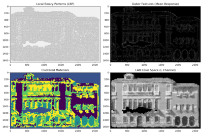
Extending the pipeline to include a detection model that identifies and localizes the missing or occluded parts of the facade. Specifically:
1) Instead of randomly masking square patches, as is common in standard Masked Autoencoder (MAE) pipelines, it is more effective to directly identify the specific regions that genuinely require inpainting. This approach ensures that the MAE focuses on reconstructing truly missing parts of the data, rather than inadvertently altering intact sections of the image. To achieve this, one can analyze the geometric properties of contours that outline potential missing areas and apply contour simplification algorithms, such as the Ramer–Douglas–Peucker (RDP) algorithm [5][6].
The RDP algorithm approximates complex contours with fewer points while retaining their essential shape. By examining the resulting simplified contours, one can distinguish between regions that are genuinely missing due to data loss and those that merely appear missing because they are obscured by other objects (such as overlapping facades) or cast shadows. Regular, smoothly simplified contours—often approximating geometric shapes like rectangles—are more likely to represent occlusions or overshadowed areas that do not require inpainting. In contrast, regions with irregular, non-uniform contours that remain complex even after RDP simplification are more plausibly true missing areas caused by experimental constraints, sensor malfunctions, or environmental factors like foliage interference. Identifying such irregular contours with RDP enables a targeted inpainting strategy that improves the quality and relevance of the reconstructed data (as in an example shown on the right).
2) By directly integrating more feature representations (as in figure shown on the right) into the Masked Autoencoder (MAE) pipeline, one can provide the model with richer priors that guide the inpainting process more effectively. For instance, instead of relying solely on raw RGB inputs, additional channels derived from Local Binary Patterns (LBP) and Gabor features can be concatenated or fused into the MAE’s encoder input. This way, the model receives explicit signals about local texture directionality, micro-structure repetitions, and edge distributions. Likewise, the LAB luminance channel offers cues on shading and brightness gradients, while material clustering maps highlight spatially coherent regions, allowing the model to group visually similar areas and maintain consistent texture and color properties within each masked patch. This multi-channel input strategy ensures the latent representations in the MAE capture both low-level textures and higher-level structural semantics, making it easier for the decoder to reconstruct missing segments accurately.
From an architectural perspective, the MAE can be adapted to process these features through parallel branches or specialized attention layers that learn to weight and blend the different modalities. By incorporating loss functions that penalize discrepancies not only in pixel space but also in the feature space (e.g., ensuring that reconstructed textures have similar LBP/Gabor statistics), the training process encourages the network to leverage these additional inputs more effectively. Furthermore, the inclusion of material segmentation maps as priors for masking strategies (e.g., preferring to mask regions that are contextually distinct in material composition) can enhance the MAE’s ability to learn robust completion patterns. Overall, these technical adaptations allow the MAE to move beyond naive pixel-level patch prediction towards a more context-aware, structure-preserving, and material-consistent inpainting approach.
3) Partial Facades: Once the model has successfully identified genuinely missing or occluded areas within the facade imagery, the trained MAE can be deployed to reconstruct these regions. Rather than relying solely on synthetic, randomly placed patches during training, employing an MAE on segments explicitly identified as missing allows the model to engage with more contextually relevant structures. For instance, if the detection model isolates irregularly shaped gaps—likely due to data loss or actual occlusions—the MAE can focus its latent representations on these specific anomalies. By doing so, the inpainting process moves beyond simple pattern replication, employing the learned embeddings to infer plausible architectural elements, color gradients, and textures that align with the global aesthetic and structural semantics of Venetian facades. Fine-tuning the MAE on partial facade datasets, which contain a range of occlusion levels and missing detail intensities, further refines the model’s ability to handle intricate architectural patterns. This additional training step encourages adaptability and robustness, enabling the MAE to produce realistic reconstructions even under challenging conditions, such as when large portions of the image remain unseen or feature subtle architectural motifs requiring careful inference.
By addressing these future directions, the MAE can be effectively utilized for practical inpainting tasks, enabling the restoration of incomplete facades while preserving architectural coherence. This would be particularly valuable for urban restoration projects, virtual reconstructions, and similar real-world applications.
References
- ↑ Ojala, T., Pietikäinen, M., & Mäenpää, T. (2002). Multiresolution grayscale and rotation invariant texture classification with Local Binary Patterns. IEEE Transactions on Pattern Analysis and Machine Intelligence, 24(7), 971–987. doi:10.1109/TPAMI.2002.1017623
- ↑ Dalal, N., & Triggs, B. (2005). Histograms of Oriented Gradients for Human Detection. 2005 IEEE Computer Society Conference on Computer Vision and Pattern Recognition (CVPR’05), Vol. 1, 886–893. doi:10.1109/CVPR.2005.177
- ↑ Gabor, D. (1946). Theory of communication. Journal of the Institution of Electrical Engineers - Part III: Radio and Communication Engineering, 93(26), 429–457. doi:10.1049/ji-3-2.1946.0074
- ↑ He, K., Chen, X., Xie, S., Li, Y., Dollár, P., & Girshick, R. (2022). Masked Autoencoders Are Scalable Vision Learners. Proceedings of the IEEE/CVF Conference on Computer Vision and Pattern Recognition (CVPR), 16000–16009. https://openaccess.thecvf.com/content/CVPR2022/papers/He_Masked_Autoencoders_Are_Scalable_Vision_Learners_CVPR_2022_paper.pdf
- ↑ Ramer, U. (1972). An iterative procedure for the polygonal approximation of plane curves. Computer Graphics and Image Processing, 1(3), 244–256. doi:10.1016/S0146-664X(72)80017-0
- ↑ Douglas, D. H., & Peucker, T. K. (1973). Algorithms for the Reduction of the Number of Points Required to Represent a Digitized Line or its Caricature. Cartographica: The International Journal for Geographic Information and Geovisualization, 10(2), 112–122. doi:10.3138/FM57-6770-U75U-7727
