Paintings / Photos geolocalisation: Difference between revisions
Yuanhui.lin (talk | contribs) |
Yuanhui.lin (talk | contribs) |
||
| (106 intermediate revisions by 3 users not shown) | |||
| Line 1: | Line 1: | ||
==Introduction== | ==Introduction== | ||
The goal of this project is to locate a given painting or photo of Venice on the map. In the final website we implement, user can upload an image, and the predicted location of the image will be shown on the map. | The goal of this project is to locate a given painting or photo of Venice on the map. We use two different methods to achieve this goal, one is to use SIFT to find matched key points of the images, the other is to use deep learning model. In the final website we implement, user can upload an image, and the predicted location of the image will be shown on the map. | ||
==Motivation== | ==Motivation== | ||
| Line 62: | Line 62: | ||
* Write project report. | * Write project report. | ||
* Prepare slides for final presentation. | * Prepare slides for final presentation. | ||
| align="center" | | | align="center" | ✓ | ||
|- | |- | ||
|By Week 14 | |By Week 14 | ||
| Line 68: | Line 68: | ||
* Finish presentation slides and report writing. | * Finish presentation slides and report writing. | ||
* Presentation rehearsal and final presentation. | * Presentation rehearsal and final presentation. | ||
| align="center" | | | align="center" | -- | ||
|- | |- | ||
|} | |} | ||
| Line 79: | Line 79: | ||
We repeat the first step for several times and realize that for each time, the number of returned images is different. We therefore processed our text files by deleting the duplicated images and merging them. Then, we use requests package to download collected images using the URLs we get from previous step, at the same time, we generate a label text file with geo-coordinates and corresponding image file names. | We repeat the first step for several times and realize that for each time, the number of returned images is different. We therefore processed our text files by deleting the duplicated images and merging them. Then, we use requests package to download collected images using the URLs we get from previous step, at the same time, we generate a label text file with geo-coordinates and corresponding image file names. | ||
Finally, we get 2387 images of Venice buildings with geo-coordinates. | Finally, we get 2387 images of Venice buildings with geo-coordinates. | ||
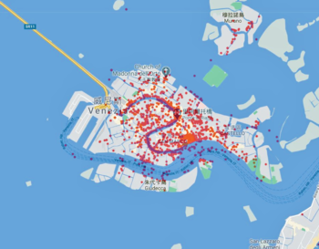
[[File:Tt.png|350px|thumb|center|Figure 1: Images Distribution]] | |||
[[File:Tt.png| | |||
===SIFT=== | ===SIFT=== | ||
| Line 99: | Line 98: | ||
===Deep Learning=== | ===Deep Learning=== | ||
The idea of using deep learning model to find the geo-coordinates of an image is inspired by [https://resources.wolframcloud.com/NeuralNetRepository/resources/ResNet-101-Trained-on-YFCC100m-Geotagged-Data Wolfram]. However, instead of using a classification method, we use regression model to predict the latitude and longitude of an image directly. We implement the model using TensorFlow Keras module provided in python. As in this module, structure of different kinds of CNN models are provided and pre-trained. This is essential since we are not sure if the data we collected is enough to train a model start from nothing. We utilize the model pre-trained on ImageNet, freeze the weights of those main layers and modify the input layer and output layer in order to make the neural network suitable for our purpose. In the training process, only the weights of the layers we modified will be updated. | |||
* '''Model Selection''' | |||
In the [https://resources.wolframcloud.com/NeuralNetRepository/resources/ResNet-101-Trained-on-YFCC100m-Geotagged-Data Wolfram] project, ResNet101 was trained on YFCC100m geo-tagged data, and is shown to have pretty satisfied predicted result. And in another [http://mi.eng.cam.ac.uk/projects/relocalisation/#results project done by Cambridge University], a modified GoogLeNet is used to predict the camera position of a given image. Therefore, when selecting model to be used in our project, we mainly try Inception models and ResNet models. | |||
{|class="wikitable" style="margin: 1em auto 1em auto;" | |||
|- | |||
!Model | |||
!Learning Curve | |||
!Predict Results | |||
!Model | |||
!Learning Curve | |||
!Predict Results | |||
|- | |||
| ResNet50 | |||
| [[File:Fan.JPG|250px|center]] | |||
| | |||
* Average distance: 727m | |||
* Min distance: 37m | |||
* Max distance: 2869m | |||
| ResNet50V2 | |||
| [[File:50v2.JPG|250px|center]] | |||
| | |||
* Average distance: 1777m | |||
* Min distance: 134m | |||
* Max distance: 11804m | |||
|- | |||
| ResNet101 | |||
| [[File:Aaa.JPG|250px|center]] | |||
| | |||
* Average distance: 695m | |||
* Min distance: 33m | |||
* Max distance: 3490m | |||
| ResNet101V2 | |||
| [[File:101v2.JPG|250px|center]] | |||
| | |||
* Average distance: 1333m | |||
* Min distance: 49m | |||
* Max distance: 8218m | |||
|- | |||
| InceptionResNetV2 | |||
| [[File:Inc.JPG|250px|center]] | |||
| | |||
* Average distance: 1633m | |||
* Min distance: 126m | |||
* Max distance: 7461m | |||
| InceptionV3 | |||
| [[File:In.JPG|250px|center]] | |||
| | |||
* Average distance: 1799m | |||
* Min distance: 28m | |||
* Max distance: 5492m | |||
|- | |||
|} | |||
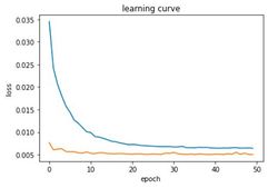
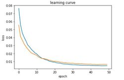
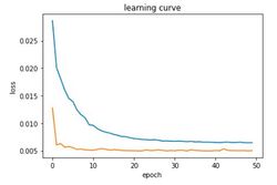
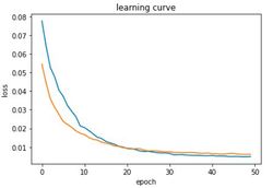
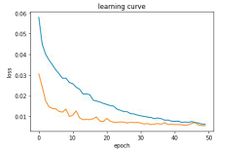
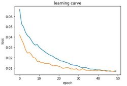
We compare the six different models and observe that ResNet50 and ResNet101 converge faster than other models, and the predict results are better. In our project, we finally choose the ResNet101 model, as given the experience from Wolfram, we think it is suitable for our purpose. | |||
* '''Fine-Tuning''' | |||
We modify the output layer of ResNet101 model to make it a regression model. In the fine-tuning process, we set epoch to be 35. | |||
We normalize latitude and longitude with different methods, add dropout layer before the final output layer and adjust the ratio of dropout, change the activation function of the output layer and use different loss functions. Finally, we choose min-max normalization of label, add a dropout layer with 0.2 dropout ratio, set activation function to be linear and use MSE as the loss function. | |||
===Web Implementation=== | ===Web Implementation=== | ||
* '''Streamlit''' | |||
For the web implementation, we used the Streamlit, an open-source app framework for Machine Learning and Data Science teams. At first we were considering to use the Django framework, but by comparison we found that the Streamlit is a more faster way in helping creating a beautiful and simple interactive data app. | |||
To see the web page effect, you need to install the Streamlit library and then download our code in the link. [https://www.streamlit.io/ Here] you can find more details about Streamlit. | |||
* '''Web interface''' | |||
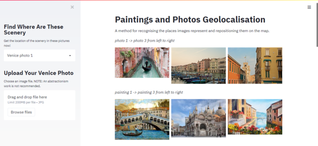
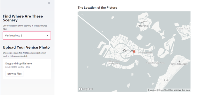
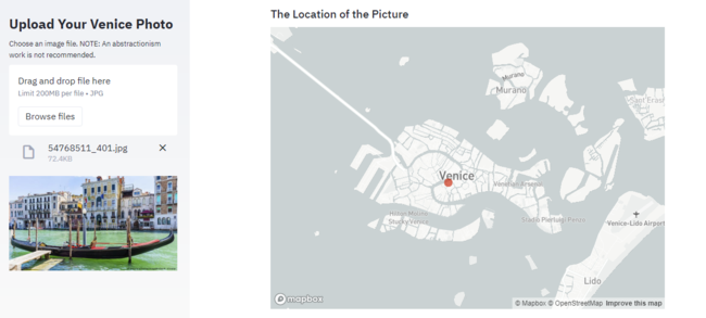
Here the app provides users with 3 sample photos and 3 sample oil paintings about Venice. Users can select the pictures in the checkbox in the sidebar to view their locations on the map. They can also upload an image file to view its position. | |||
[[File:Web 1.png|650px|thumb|center|Figure 2: Web interface screenshot(1)]] | |||
The map shows the location of "Venice photo 3". | |||
[[File:Web 2.png|650px|thumb|center|Figure 3: Web interface screenshot(2)]] | |||
The map shows the location of the picture uploaded by the user. | |||
[[File:Web 3.png|650px|thumb|center|Figure 4: Web interface screenshot(3)]] | |||
==Assessment== | ==Assessment== | ||
===''' | ===Sift Results=== | ||
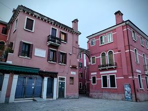
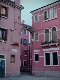
* '''Sample of matching results''' | |||
[[File:1625.jpg| | {|class="wikitable" style="margin: 1em auto 1em auto;" | ||
|- | |||
| [[File:1625.jpg|300px|thumb|center]] | |||
| [[File:1587.jpg|200px|thumb|center]] | |||
|- | |||
| [[File:1613.jpg|300px|thumb|center]] | |||
| [[File:1545.jpg|300px|thumb|center]] | |||
|- | |||
| [[File:583.jpg|300px|thumb|center]] | |||
| [[File:573.jpg|300px|thumb|center]] | |||
|- | |||
| [[File:1031.jpg|300px|thumb|center]] | |||
| [[File:1030.jpg|300px|thumb|center]] | |||
|} | |||
* '''Distribution of MSE''' | |||
We try to visualize the kernel density estimation and histogram of the MSE to see how it distributes. | |||
{|class="wikitable" style="margin: 1em auto 1em auto;" | |||
|- | |||
|[[File:Error_distribution.png|300px|thumb|center|Figure 5: MSE kdeplot]] | |||
|[[File:Distplot_of_MSE.png|300px|thumb|center|Figure 6: MSE distplot]] | |||
|} | |||
* '''Bootstrapping''' | |||
Because we do not have a large enough dataset, we try to use a bootstrapping method to detect the distribution of median value of MSE. We set a 10000-loop bootstrapping and find the 95% CI of the median value is [1.198612000000505e-05, 9.385347600000349e-05] and 50% CI is [3.817254499999426e-05, 6.0381709000008324e-05]. Combined with our visualization results, we estimate that the mean MSE of Sift geolocalisation is of about e-05 order of magnitude, which means the mean distance error is of about km order of magnitude. | |||
===Deep Learning Results=== | |||
* '''Objective Evaluation''' | |||
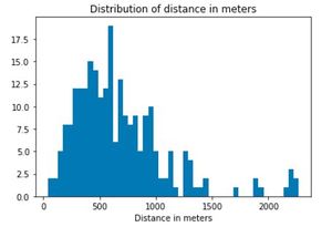
We test our model with randomly selected 10% images from our image dataset, which is different from the training dataset. We draw the distribution of difference in predict location and actual location in meters. The average difference in distance is ~700m, with minimum distance <100m and maximum distance <3000m. | |||
[[File:Distribution.JPG|300px|thumb|center|Figure 7: Distance Distribution]] | |||
* '''Subjective Evaluation''' | |||
We implement a website where the map of Venice is shown. One can upload an image with known geo-location and see how different the predict location can be compared with the correct location. This can give a brief idea of how accurate the model is. | |||
==Limitation== | |||
The two methods we use have some limitations. | |||
For the SIFT method, although the accuracy seems to be high, this method take quite a long time to find the location of an image, as for each input image we traverse all the images in the database to find the best match. With more than 2000 images, it takes around 3 minutes to find the best match (this timing is different for different machines), which is too long for us to implement this method on the website. Also, the accuracy highly depend on the images we have in the dataset. Only if we have images of every corner of Venice can we identify the location of a random image input correctly. However, with more images in dataset, the consuming time will grow as well. | |||
For the deep learning method, as shown in the assessment, the result is not very satisfying with an average distance error of ~700m. When we discuss about the possible reasons, we think one is that the dataset is not large enough. As one can see the distribution of images in Figure1, most of the images we collected are along the canal and in San Marco, this may cause imbalance of data. Also, we are not sure if regression model is reasonable to predict the latitude and longitude. | |||
==Future Work== | ==Future Work== | ||
===Multiprocessing Sift=== | |||
Our sift matching method is time-consuming. We tested 47 images and it cost about 3 minute to find the most similar image for each image. If we have larger matching dataset, this method may not perform well because of the long processing time. We have tried simple CPU multiprocessing, but the result did not improve dramatically. So we may consider other multiprocessing method and some special data structure to store the sift descriptor, which may contribute to a shorter matching time. | |||
===Resnet Classification=== | |||
For our deep learning method, we try to give the geo-coordinates by regression. Inspired by a geolocation model classifies the location offered by Wolfram, we are considering if a classification model can have a better results. We can simply use our own grid to assigned each image to a certain cluster. Furthermore, Google offers the S2 Geometry Library, which represents all data on a three-dimensional sphere (similar to a globe). This makes it possible to build a worldwide geographic database with no seams or singularities, using a single coordinate system, and with low distortion everywhere compared to the true shape of the Earth. It offers different level of cells whose average area ranges from 85011012.19 km2 to 0.74 cm2. With S2 library, each image can be assigned to a cell. Then we can train our geolocation classfication model. However, how to choose a proper level of cell to get the best results need more experiments. | |||
===Multi-source Data=== | |||
Currently, we do not have a large dataset of images with geo-coordinates. We may try to get more geo-tagged images from other social media like facebook, instagram or something else. We can also give an access to users to upload images with geo-coordinates. However, there is still a problem to be solved that for this type of multisource dataset, how we can check the accuracy of their geo-coordinates? And this effects our results dramatically. | |||
==Links== | ==Links== | ||
| Line 124: | Line 237: | ||
#[https://aws.amazon.com/blogs/machine-learning/estimating-the-location-of-images-using-mxnet-and-multimedia-commons-dataset-on-aws-ec2/ Estimating the Location of Images Using Apache MXNet and Multimedia Commons Dataset on AWS EC2] | #[https://aws.amazon.com/blogs/machine-learning/estimating-the-location-of-images-using-mxnet-and-multimedia-commons-dataset-on-aws-ec2/ Estimating the Location of Images Using Apache MXNet and Multimedia Commons Dataset on AWS EC2] | ||
#[https://resources.wolframcloud.com/NeuralNetRepository/resources/ResNet-101-Trained-on-YFCC100m-Geotagged-Data Wolframe Neural Net Repository] | #[https://resources.wolframcloud.com/NeuralNetRepository/resources/ResNet-101-Trained-on-YFCC100m-Geotagged-Data Wolframe Neural Net Repository] | ||
#[http://mi.eng.cam.ac.uk/projects/relocalisation/#results Visual Localisation project from University of Cambridge] | |||
Latest revision as of 21:48, 16 December 2020
Introduction
The goal of this project is to locate a given painting or photo of Venice on the map. We use two different methods to achieve this goal, one is to use SIFT to find matched key points of the images, the other is to use deep learning model. In the final website we implement, user can upload an image, and the predicted location of the image will be shown on the map.
Motivation
Travelling is nowadays a universal hobby. There are many platforms like Instagram and Flickr for people to post their travel photos and share with strangers. With geo information of the posts provided by bloggers, other users can search pictures in a specific location and decide if they want to go travel there. But how about seeing an amazing picture without location indicated? We would like to address this problem in our project. We hope to come up with a solution that can locate an image on map so that if someone find a gorgeous picture without geo information, he or she can use our method to find the location of the place and plan a trip there.
Also, our method should work on realistic paintings, as the features in those painting should be similar as in photo. Therefore, art lovers can use our method to locate a painting and be in the painting themselves.
The scale is restricted to Venice in our project.
Project Plan and Milestones
| Date | Task | Completion |
|---|---|---|
| By Week 3 |
|
✓ |
| By Week 8 |
|
✓ |
| By Week 9 |
|
✓ |
| By Week 10 |
|
✓ |
| By Week 11 |
|
✓ |
| By Week 12 |
|
✓ |
| By Week 13 |
|
✓ |
| By Week 14 |
|
-- |
Methodology
Data collection
We use the python package flickrapi to crawl photos with geo-coordinates inside Venice from Flickr. In order to exclude the photos of events and human portrait that are taken in Venice, we set the key words to be "Venice, building". Since it is possible that the keyword "Venice" appear in photos taken in other place, we also set up a latitude and longitude region of Venice, returned photos with geo-coordinates outside this range will not be considered. After this step, we generate a text file containing the geo-coordinates of photos and URLs to the photos.
We repeat the first step for several times and realize that for each time, the number of returned images is different. We therefore processed our text files by deleting the duplicated images and merging them. Then, we use requests package to download collected images using the URLs we get from previous step, at the same time, we generate a label text file with geo-coordinates and corresponding image file names.
Finally, we get 2387 images of Venice buildings with geo-coordinates.
SIFT
SIFT, scale-invariant feature transform, is a feature detection algorithm to detect and describe local features in images. We try to use this method to detect and describe key points in the image to be geolocalised and images with geo-coordinates. With these key points, we can find the most similar image and then finish the geolocalisation.
- Dataset spliting
To check the feasibility of our method, we try to use images with geo-coordinates to test. Therefore, we should split our dataset into testing dataset(to find geo-coordinates) and matching dataset(with geo-coordinates). In our experiment, because we do not have a dataset large enough and the matching without parallel is time-consuming, we randomly choose 2% of the dataset to be test dataset.
- Scale-invariant feature detection and description
We should firstly project the image into a collection of vector features. The keypoints defined thoes who has local maxima and minima of the result of difference of Gaussians function in the vector feature space, and each keypoint will have a descriptor, including location, scale and direction. This process can be simply completed with the python lib CV2.
- Keypoints matching
To find the most similar image with geo-coordinates, we do keypoints match for each test image, finding the keypoint pairs with all images in the matching dataset. Then, calculating the sum distance of top 50 matched pairs' distance. We choose the image with the smallest sum distance as the most similar image and give its geo-coordinates to the test image.
- Error analysis
For each match-pair, we calulate the MSE(mean square error) of lantitude and longitude. In order to assess our result, We try to visualise the distribution of MSE and give a 95% CI of median value of MAE by bootstrapping.
Deep Learning
The idea of using deep learning model to find the geo-coordinates of an image is inspired by Wolfram. However, instead of using a classification method, we use regression model to predict the latitude and longitude of an image directly. We implement the model using TensorFlow Keras module provided in python. As in this module, structure of different kinds of CNN models are provided and pre-trained. This is essential since we are not sure if the data we collected is enough to train a model start from nothing. We utilize the model pre-trained on ImageNet, freeze the weights of those main layers and modify the input layer and output layer in order to make the neural network suitable for our purpose. In the training process, only the weights of the layers we modified will be updated.
- Model Selection
In the Wolfram project, ResNet101 was trained on YFCC100m geo-tagged data, and is shown to have pretty satisfied predicted result. And in another project done by Cambridge University, a modified GoogLeNet is used to predict the camera position of a given image. Therefore, when selecting model to be used in our project, we mainly try Inception models and ResNet models.
| Model | Learning Curve | Predict Results | Model | Learning Curve | Predict Results |
|---|---|---|---|---|---|
| ResNet50 |
|
ResNet50V2 |
| ||
| ResNet101 |
|
ResNet101V2 |
| ||
| InceptionResNetV2 |
|
InceptionV3 |
|
We compare the six different models and observe that ResNet50 and ResNet101 converge faster than other models, and the predict results are better. In our project, we finally choose the ResNet101 model, as given the experience from Wolfram, we think it is suitable for our purpose.
- Fine-Tuning
We modify the output layer of ResNet101 model to make it a regression model. In the fine-tuning process, we set epoch to be 35.
We normalize latitude and longitude with different methods, add dropout layer before the final output layer and adjust the ratio of dropout, change the activation function of the output layer and use different loss functions. Finally, we choose min-max normalization of label, add a dropout layer with 0.2 dropout ratio, set activation function to be linear and use MSE as the loss function.
Web Implementation
- Streamlit
For the web implementation, we used the Streamlit, an open-source app framework for Machine Learning and Data Science teams. At first we were considering to use the Django framework, but by comparison we found that the Streamlit is a more faster way in helping creating a beautiful and simple interactive data app.
To see the web page effect, you need to install the Streamlit library and then download our code in the link. Here you can find more details about Streamlit.
- Web interface
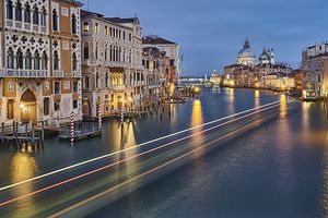
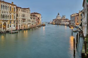
Here the app provides users with 3 sample photos and 3 sample oil paintings about Venice. Users can select the pictures in the checkbox in the sidebar to view their locations on the map. They can also upload an image file to view its position.
The map shows the location of "Venice photo 3".
The map shows the location of the picture uploaded by the user.
Assessment
Sift Results
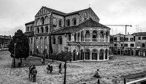
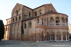
- Sample of matching results
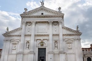
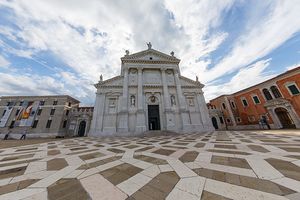
- Distribution of MSE
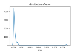
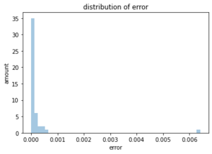
We try to visualize the kernel density estimation and histogram of the MSE to see how it distributes.
- Bootstrapping
Because we do not have a large enough dataset, we try to use a bootstrapping method to detect the distribution of median value of MSE. We set a 10000-loop bootstrapping and find the 95% CI of the median value is [1.198612000000505e-05, 9.385347600000349e-05] and 50% CI is [3.817254499999426e-05, 6.0381709000008324e-05]. Combined with our visualization results, we estimate that the mean MSE of Sift geolocalisation is of about e-05 order of magnitude, which means the mean distance error is of about km order of magnitude.
Deep Learning Results
- Objective Evaluation
We test our model with randomly selected 10% images from our image dataset, which is different from the training dataset. We draw the distribution of difference in predict location and actual location in meters. The average difference in distance is ~700m, with minimum distance <100m and maximum distance <3000m.
- Subjective Evaluation
We implement a website where the map of Venice is shown. One can upload an image with known geo-location and see how different the predict location can be compared with the correct location. This can give a brief idea of how accurate the model is.
Limitation
The two methods we use have some limitations.
For the SIFT method, although the accuracy seems to be high, this method take quite a long time to find the location of an image, as for each input image we traverse all the images in the database to find the best match. With more than 2000 images, it takes around 3 minutes to find the best match (this timing is different for different machines), which is too long for us to implement this method on the website. Also, the accuracy highly depend on the images we have in the dataset. Only if we have images of every corner of Venice can we identify the location of a random image input correctly. However, with more images in dataset, the consuming time will grow as well.
For the deep learning method, as shown in the assessment, the result is not very satisfying with an average distance error of ~700m. When we discuss about the possible reasons, we think one is that the dataset is not large enough. As one can see the distribution of images in Figure1, most of the images we collected are along the canal and in San Marco, this may cause imbalance of data. Also, we are not sure if regression model is reasonable to predict the latitude and longitude.
Future Work
Multiprocessing Sift
Our sift matching method is time-consuming. We tested 47 images and it cost about 3 minute to find the most similar image for each image. If we have larger matching dataset, this method may not perform well because of the long processing time. We have tried simple CPU multiprocessing, but the result did not improve dramatically. So we may consider other multiprocessing method and some special data structure to store the sift descriptor, which may contribute to a shorter matching time.
Resnet Classification
For our deep learning method, we try to give the geo-coordinates by regression. Inspired by a geolocation model classifies the location offered by Wolfram, we are considering if a classification model can have a better results. We can simply use our own grid to assigned each image to a certain cluster. Furthermore, Google offers the S2 Geometry Library, which represents all data on a three-dimensional sphere (similar to a globe). This makes it possible to build a worldwide geographic database with no seams or singularities, using a single coordinate system, and with low distortion everywhere compared to the true shape of the Earth. It offers different level of cells whose average area ranges from 85011012.19 km2 to 0.74 cm2. With S2 library, each image can be assigned to a cell. Then we can train our geolocation classfication model. However, how to choose a proper level of cell to get the best results need more experiments.
Multi-source Data
Currently, we do not have a large dataset of images with geo-coordinates. We may try to get more geo-tagged images from other social media like facebook, instagram or something else. We can also give an access to users to upload images with geo-coordinates. However, there is still a problem to be solved that for this type of multisource dataset, how we can check the accuracy of their geo-coordinates? And this effects our results dramatically.
Links
Paintings/Photos geolocalisation GitHub
