Opera Rolandi archive: Difference between revisions
| (91 intermediate revisions by 2 users not shown) | |||
| Line 2: | Line 2: | ||
== Abstract == | == Abstract == | ||
The Fondazione Giorgio Cini has digitized 36000 pages from Ulderico Rolandi's opera [http://dl.cini.it/collections/show/1120 | The Fondazione Giorgio Cini has digitized 36000 pages from Ulderico Rolandi's opera [http://dl.cini.it/collections/show/1120 libretti collection]. This collection contains contemporary works of 17th- and 18th-century composers. These opera libretti have a diverse content, which offers a large amount of possibilities for analysis. | ||
This project concentrates on a way to illustrate the characters’ interactions in the Rolandi's libretti collection through network visualization as well as the importance of each character in the acts they figure in. To achieve this, we retrieved important information using the DHLAB Deep Learning model [https://github.com/dhlab-epfl/dhSegment-torch | This project concentrates on a way to illustrate the characters’ interactions in the Rolandi's libretti collection through network visualization as well as the importance of each character in the acts they figure in. To achieve this, we retrieved important information using the DHLAB Deep Learning model [https://github.com/dhlab-epfl/dhSegment-torch dhSegment-torch] and [https://cloud.google.com/vision/docs/ocr Google Vision OCR]. We started from one opera libretto of Rolandi’s libretti collection, [http://dl.cini.it/collections/show/333 Antigona] with RecordID MUS0030011 and generalized it to another libretto, [http://dl.cini.it/collections/show/435 Gli americani] with RecordID MUS0010824. | ||
== | == Description of the methods == | ||
=== Motivation === | |||
Our initial motivation was to create using all the Rolandi's libretti collection a timeline visualization of the opera's literary movements. As each movement has its own themes and characteristics, we wanted to extract, using OCR and NLP methods, the most common topics of each libretto and propose them as new metadata to the Fondazione Giorgio Cini. As the NLP algorithms are greatly accurate on English texts, we wanted to first translate each libretto from italian to english using Linguee's [https://www.deepl.com/translator DeepL tool]. There we encountered the problem which didn't permit to further permit the extraction of the complete texts. | |||
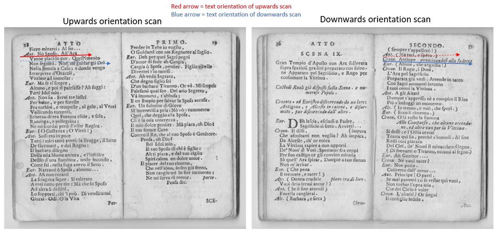
Indeed, as the digital images have different orientations due to the scanning, it was difficult to rearrange the words of our libretto into the correct sentences based uniquely on the x and y coordinates of the boxes surrounding our words. Different solutions have been proposed, like grouping the vertical coordinates into bins to reflect the sentences boxes, but this won't work as it still depends on the orientation of the document (one sentence can go upwards or downwards, depending on if the book is slightly turned upwards or downwards). | |||
[[File:OrientationScans.JPG|1000px|center|thumb|Orientation of texts in different scans]] | |||
The second problem that we encountered is the complexity of the scraping of the libretti. First the time to extract each page scan from one libretto of the collection is significant and defining which important pages to keep for the analysis (only the pages where the story content figures and removing the pages containing metadata) was difficult. | |||
Therefore we shifted the direction of our project's goal and settled on the creation of a visualization tool to illustrate the evolution of the characters’ interactions and importance per libretto. This type of network analysis is way more interesting as already showed in the paper [https://www.google.com/url?sa=t&rct=j&q=&esrc=s&source=web&cd=&ved=2ahUKEwik_8uNsMjtAhVPLewKHcZPDAIQFjAAegQIAhAC&url=https%3A%2F%2Flitlab.stanford.edu%2FLiteraryLabPamphlet2.pdf&usg=AOvVaw0NBU1pFLlEuji0fNHhH6D_ Literary Lab Pamphlet 2] by Franco Moretti, one of the many series of studies done at the Stanford Literary Lab on how to quantify novels or plays. | |||
For now, the goal of the project is to focus on a small subset of the Rolandi's libretti collection to ensure the creation of an accurate tool. With this project, we hope to provide an additional tool for anyone wanting to analyse opera's libretti, and especially the relationship between its characters. Ultimately, using this tool on a larger set of libretti could potentially help understanding some underlying structure behind opera's logic, and give some insight on past opera's culture. | |||
== | === Dataset === | ||
[ | We had access to the archives of the Cini Foundation in Venice, which holds around [http://dl.cini.it/collections/show/1120 32 000 digitized opera's libretti]. | ||
To train our deep learning model for it to perform accurately, we need to choose and segment a lot of different formats of libretti's images. We therefore randomly choose Rolandi's libretti and select random pages from them for training and validation. There are a total of 34 training images, 12 validation images and several testing images. | |||
We decided to first focus on one libretto with which we're going to test our complete model and test our visualization tool. The libretto needs to have an easy and helpful format for the extraction of the abbreviation names, scenes and descriptions of the scenes in the segmentation part. The text thus has to be sufficiently readable and interspaced. This brought us to the choice of the libretto [http://dl.cini.it/collections/show/333 Antigona, MUS0030011]. One has to keep in mind that the model hyperparameters' tuning and elaboration of concepts for extracting the relationship network were all done based on this libretto. | |||
To be able to test our model accuracy, we need to try to at least use the implemented tool on another libretto which the deep learning model has never encountered. We therefore randomly choose the [http://dl.cini.it/collections/show/435 Gli americani, MUS0010824] for testing the generalization of our tool. | |||
=== Segmentation === | |||
As explained before, the orientation of the images' scans bring a lot of difficulties in the analysis of the dialogues, as the text can be wrongly reordered and thus impact the logical ordering of the discussions. Therefore, for measuring the weight of importance of a character and the weight of its relationship with another character, we need to select a measuring method. First, we decide to extract the abbreviations names figuring in the beginning of a dialogue and which illustrate which characters is speaking the next sentences. Unfortunately, these names are not complete, and thus we need to infer the complete name of the character using the description section below each scene, which has the role of mentionning the place of the scene and the characters complete names taking part in it. This description section is therefore useful for linking the extracted abbreviation names with their complete version. | |||
Then, to be able to bring a timeline into this analysis, we include the acts and scenes which are the important time and space delimiters of a play or opera. Therefore we focus only on the extraction of the scenes, as one can infer at which moment the new act begins based on the value of the scene. | |||
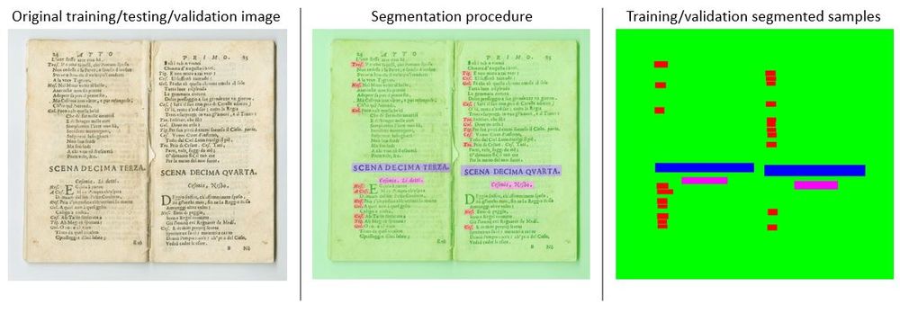
To define which words belong to which of the defined classes (scenes, descriptions or abbreviation names), we use the DHLAB deep learning pre-trained model, [https://paperswithcode.com/paper/dhsegment-a-generic-deep-learning-approach#code dh-segment]. This model needs as an input segmented images which uniquely color the elements in the image corresponding to a certain attribute. This color schema has to be reused in all the training and validation samples as to be able to extract the probability of a pixel of the image to belong to some particular class. This list of class probabilities has the same length as the image from which the words have been extracted, thus the extraction of the words is feasible. | |||
Below, we can find an example of how the segmentation has been done on our training and validation images. | |||
[[File:Segmentation.JPG|1000px|center|thumb|Segmentation used for extraction of words per attribute]] | |||
=== OCR === | |||
For the extraction of the text words and the box' coordinates surrounding the corresponding word in our libretti's scans, we use the [https://cloud.google.com/vision/docs/ocr Google Vision API] which already offers an OCR tool to detect text in images. | |||
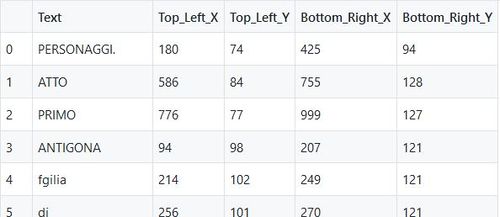
We decided to store the words and some of the box' coordinates in a csv file (in the order of detection). We therefore store the top left x coordinate, which is as well the bottom left x coordinate, the top left y coordinate (= top right y coordinate), the bottom right x coordinate (= top right x coordinate) and the bottom right y coordinate (= bottom left coordinate). Therefore we store in an efficient way all the important coordinates to recreate the box where the word has been detected in the text. This csv file will be helpful to reorder the extracted elements in the correct order of appearance (in the way a human reads a book). | |||
=== | |||
[[File:StoredCoordinates.JPG|500px|center|thumb|CSV file of stored words and respective coordinates]] | [[File:StoredCoordinates.JPG|500px|center|thumb|CSV file of stored words and respective coordinates]] | ||
=== Combination of OCR and | === Combination of OCR and segmentation to find words of interest === | ||
Using the prediction classes probabilities for each pixel of the image | Using the prediction classes' probabilities for each pixel of the image which were computed using dh_segment, we can now create a mask to extract the words belonging to these classes. | ||
As the probability is distributed among all classes, one has to define an ocr_threshold which specifies at which point one pixel of the image belongs to one class. This 1 and 0 values will be stored as a mask for each attribute. | As the probability is distributed among all classes, one has to define an ocr_threshold which specifies at which point one pixel of the image belongs to one class. This 1 and 0 values will be stored as a mask for each attribute. | ||
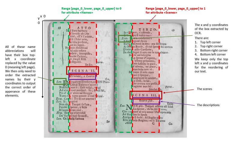
We define a range of the image from which to extract the words for each attribute (i.e. for the extraction of the names, we want to extract in the most left part of the left page, and the most left part of the right page.). We use this trick for two | We define a range of the image from which to extract the words for each attribute (i.e. for the extraction of the names, we want to extract in the most left part of the left page, and the most left part of the right page.). We use this trick for two reasons: first, this helps us order our words, finding the ones from the first page and then the ones form the second page, and second to optimize our algorithm so that it doesn't go through all the image, and saves us an important amount of time. We however choose a quite large range so that we are sure we do not miss any data. The picture below illustrates this. | ||
[[File:AttributesPages.JPG|800px|center|thumb|OCR procedure and Attributes extraction]] | [[File:AttributesPages.JPG|800px|center|thumb|OCR procedure and Attributes extraction]] | ||
Then, | Then, we focus on a word and its particular box. We compute the mean of the class probability of all the pixels figuring in a smaller ratio of the box, which is centered in the true box. We don't read all the pixels of the box as the pixels further away from the center of the box have less chance of being in the class, and because at the end only the center ones matter to now if we need to keep the text in the box or not. This allows us to have a better precision on our results and gain some time. | ||
We then compute the mean value of the corresponding pixels in the OCR result - that, recall, were either 0 or 1. We define a mean_threshold for each attribute which specifies at which point the word in the box is kept as being part of the class. We will only keep these words for our analysis | [[File:OCR_seg_box.png|600px|center|thumb|Illustration of the box from the OCR transferred onto the segmentation results]] | ||
We then compute the mean value of the corresponding pixels in the OCR result - that, recall, were either 0 or 1. We define a mean_threshold for each attribute which specifies at which point the word in the box is kept as being part of the class. We will only keep these words for our analysis. | |||
After that, we return for each extracted word that matters to us their top left box x and y coordinate, that we got from the OCR results. | After that, we return for each extracted word that matters to us their top left box x and y coordinate, that we got from the OCR results. | ||
We first order the words based on their x coordinates | We first order the words based on their x coordinates and allocate them to 0 if they're in the left page, respectively 1 for the right page. This is done using the defined ranges of the image from which to extract the words for each attribute. Then we order the words based on the y coordinates from top to bottom. | ||
In the end, we have for each page the extracted words and their respective attribute affiliation (name, scene, description) in the order of appearance. | |||
=== Creating the network of a libretto === | |||
[[File:Space_scene_example.png|300px|right|thumb|Example of a spaced 'SCENA']] | |||
From the list of all the ordered attributes of the libretto, we want to create a network that will be used to visualize the relationships between the characters in time. There are many challenges here. | From the list of all the ordered attributes of the libretto, we want to create a network that will be used to visualize the relationships between the characters in time. There are many challenges here. | ||
| Line 139: | Line 80: | ||
Let's start with the problem of retrieving the names. In the dialogues, there are only abbreviations indicating which character is talking. We would want to find the full name of course. Luckily, in the description just below each scenes, there is a small text describing the place, and which characters play in the scene, by their complete name. We use this fact to find back the full name from the abbreviations. | Let's start with the problem of retrieving the names. In the dialogues, there are only abbreviations indicating which character is talking. We would want to find the full name of course. Luckily, in the description just below each scenes, there is a small text describing the place, and which characters play in the scene, by their complete name. We use this fact to find back the full name from the abbreviations. | ||
We proceed the following way : first, with all the abbreviations we found, we create a pattern, that we will use to match the full name. For example, if we have ''Ant'' we will create a pattern ''An.*t*.'', and if we have ''Aut'' we will get ''Au.*t*.''. We try to match them with words that appeared in the | We proceed the following way : first, with all the abbreviations we found, we create a regular expression pattern, that we will use to match the full name. For example, if we have ''Ant'' we will create a pattern ''An.*t*.'', and if we have ''Aut'' we will get ''Au.*t*.''. We try to match them with words that appeared in the description fields. The pattern means that we look for a word that begins with ''An'' followed by zero or many random characters followed by ''t'' followed by zero or more random characters. Once we found the full name for every abbreviations, a problem still remains : we might get some variants of the same full name, for example ''Antigona'' or ''Autigona'' ! | ||
Because the OCR might have detected variants of the same name, we need to clean that. We could first think of clustering with K-means for example, but this doesn't work because we don't know a-priori the number of clusters, which corresponds to the number of characters in the libretto. There exists techniques such as K-metroids that could be a possible solution, but we would have to think a bit about how to implement it for strings. Because of time constraints, we choose another approach : similarity distances, and in our case the edit distance from Levenstein. This distance counts the number of edits (deletion, addition, replacement) between two strings, and if it is equal or less than two, we decide that they refer to the same name. For example, ''Antigona'' and ''Autigona'' would be of a distance of one, and thus grouped together. But then we need to decide which name is the true one. We do that by selecting the one that appears the most often in the whole libretto, assuming that the OCR would be right most of the time. | |||
For the scenes, we face another problem. We need a way to correctly count and order them. The acts each start with the ''SCENA PRIMA'', meaning first scene. Then again for every act, the very last scene is ''SCENA ULTIMA''. Moreover, the scenes are counted using roman numbers. Simply extracting the number is complicated for several reasons: first, we would need to find back the index corresponding to the roman number. This could probably be done using a dictionary that maps the values. However, there is a second problem : because the typology of the scenes is very spaced (see figure on the right), the OCR considers sometimes that each letter composing the number is a different word. We then have again one of our first problem: reordering the extracted words correctly based on the scanning orientation. | |||
So we need to find another algorithm to do that. We observe that the OCR detected quite well the ''SCENA'' term. We will assume that every time we find a scene tagged ''SCENA'' or its variants ''SCEN'' or ''SCENO'', we increment the counter of scenes and add a new scene at this place. To find where a new act begins, and thus where to start the counter over, we simply look for an occurence of a scene tagged ''PRIMA''. This will define where an act starts. | |||
So we need to find another algorithm to do that. We observe that the OCR detected quite well the ''SCENA''. We will assume that every time we find a scene tagged ''SCENA'', we increment the counter of scenes and add a new scene at this place. To find where a new act | |||
Finally, with all this, we get a tree where we have the acts, scenes, names of characters appearing in the scenes and their number of occurrences in the scene. | Finally, with all this, we get a tree where we have the acts, scenes, names of characters appearing in the scenes and their number of occurrences in the scene. | ||
The tree would look something like this : | |||
[[File:tree_example.png|600px|center|thumb|Structure of The Network Tree]] | |||
=== Graph Representation of the Network === | === Graph Representation of the Network === | ||
Now that we have the tree of the libretto, we can build our network visualization. | Now that we have the tree of the libretto, we can build our network visualization. | ||
We create an interractive graph using D3.js | We create an interractive graph using [https://d3js.org D3.js]. Most of the code comes from [https://bl.ocks.org/steveharoz/8c3e2524079a8c440df60c1ab72b5d03 here]. | ||
We need to tweak a bit our previous tree to format it in the following way : | We need to tweak a bit our previous tree to format it in the following way : | ||
* A key "nodes" which contains: | * A key "nodes" which contains: | ||
** key id, the name of the character | ** key id, the name of the character | ||
** key act_N: the weight of the node, being the number of times the character appeared in the act N. There are N | ** key act_N: the weight of the node, being the number of times the character appeared in the act N. There are N keys "act", depending of the number of acts figuring in the libretto. | ||
* A key "links" which contains: | * A key "links" which contains: | ||
** key source, a character name | ** key source, a character name | ||
** key target, another character name | ** key target, another character name | ||
** key act_N: the weight of the link, being the number of scenes where the source and target characters appear together. There are N | ** key act_N: the weight of the link, being the number of scenes where the source and target characters appear together. There are N keys "act", depending of the number of acts figuring in the libretto. | ||
That way, we can visualize the importance of each character and each link between the characters, by looking at the size of the node or link. | That way, we can visualize the importance of each character and each link between the characters, by looking at the size of the node or link. | ||
You can also choose which libretto and acts you want to visualize. | You can also choose which libretto and acts you want to visualize. | ||
Here is the example of the network of Antigone : | Here is the example of the network of Antigone : | ||
[[File:antigone_network.png|400px|center|thumb|Antigone's Character's Interactions]] | |||
We see that in the | We see that in the whole libretto, all the characters interact together and we can tell which character are more important than others by looking at the size of their nodes and links. | ||
=== Generalization === | === Generalization === | ||
We now try to see how our full pipeline generalizes to other | We now try to see how our full pipeline generalizes to other libretti. We choose, arbitrarily, [http://dl.cini.it/collections/show/435; Gli americani] libretto. | ||
Here is what we got : | Here is what we got : | ||
[[File:antigone_gli.png|400px|center|thumb|Antigone's Character's Interactions]] | |||
We | We see that our algorithm works, but is a bit less good than on Antigone. This is mainly because of the hyperparameters that we previously chose to fit best the Antigone libretto. For example, abbreviations were on the images really close to the text, which made us extract words from the dialogue as names. We overfitted on Antigone, which leads to some noise in the final Gli network. For example, 'ZemEd' is not a character is the libretto. | ||
Nevertheless, we have results and more importantly we got a full pipeline that can be very easily re-used for every other libretto, to automatically find the relationships between the characters, and get some more insight about a libretto. | |||
== Quality Assesment == | == Quality Assesment == | ||
[[File:ExtractionAttributes.JPG|1200px|center|thumb| | First, let's analyse how well the segmentation model worked. Our best model has a mean Intersection Over Union of 0.55. This could have been improved with more training and validation data, and the number is not very high because of the very diverse nature of the libretto. There are as many layouts/formats as different libretto. | ||
[[File:libretti_exs.png|1200px|center|thumb|Some example of different libretti]] | |||
It still worked nicely on the Antigone's libretto that we chose : | |||
[[File:ExtractionAttributes.JPG|1200px|center|thumb|Extraction of attributes on an Antigone page]] | |||
We also analyse the overall result of our algorithm. To do that, we write by hand the real tree associated to the two libretto we tested on. This will constitute our ground truth. We use the zss algorithm and library, explained in this [http://www.grantjenks.com/wiki/_media/ideas:simple_fast_algorithms_for_the_editing_distance_between_tree_and_related_problems.pdf paper], that computes the edit distance between two trees. The edit distance is the number of modifications we need to perform to transform a tree into another. | |||
We computed the total edit distance between our extracted tree structure libretto and the ground truth, to get an overall score of how well we did. We also computed per each act the edit distances between our extracted tree structure libretto and the ground truth one. Indeed, we assume that we get a high edit distance whenever our model forgot/added a wrong scene, which will then shift the values of the nodes (i.e. the scene value) in the tree structure by 1 and thus count the children of the tree (being the characters) as being wrong. Therefore this plot will point at the extra added/removed scene. We also plot the error scene by scene. | |||
== | Let's analyse the results we got. | ||
[[File:Results_antigone_2.png|400px|center|thumb|Antigone and tree distance by act and scene]] [[File:Results_gli_2.png|400px|center|thumb|Gli and tree distance by act and scene]] | |||
We see that Antigone has a distance error of 48 and Gli of 258. This is coherent with our first view of the network data. Antigone seemed correct and Gli had more noise into it. We can look more in details at the graphs. For Antigone, we see that there is never a distance greater than 4, except for one big spike in the red act (it is the third one). To understand this, we look at the network and we see that our algorithm missed the 6th scene ! | |||
The error plot for Gli has much higher errors, and that is because the segmentation was not very accurate which leads the algorithm to fail to group correctly the names and abbreviations, and mess up the scenes | |||
== Conclusions == | |||
In conclusion of this project, we managed to read the names and scenes from a digitized libretto. We then arranged the data in a comprehensible and logic way, to finally display it as a network. In the network, we found a way to illustrate the weight of relationships between characters, along with their evolution over time. | |||
We therefore achieved our goal to implement a visualization tool for the evolution of characters' relationships in operas. This work was very focused on one specific libretto - Antigona - and does not generalize well, but we believe that improvements can be made that go into that direction. | |||
== Further research == | |||
We successfully did a first attempt at automatically analyzing the character's relationships in a libretto, from digitized images of it. However, it is far from being perfect. | |||
Here are a few ideas that may move the project forward: | |||
* Improve the segmentation model. We saw that the segmentation model was not performing extremely well because of the large range of different libretti' formats. To make it better, we should train it on more images which need to be more diverse. This would improve its accuracy and as a consequence the one of the whole algorithm. | |||
* Optimizing the hyperparameters automatically. We only did this manually, and we now have a way to measure how well our algorithm did at producing the graph. We could minimize this error over more libretti with respect to the hyperparameters by performing a grid-search on these values. This would allow even better generalization. | |||
* Creating our own distance metric between two libretti's tree. We are using a general algorithm that compares two trees. It could be nice to have a metric that reflects actually how we want to penalize forgetting an act, a scene, a character, ... | |||
==Links== | ==Links== | ||
* [https://github.com/arobaselisa/FDH-Rolandi Github repository] | |||
* [https://arobaselisa.github.io/FDH-Rolandi/ Website of the interactive relationship network vizualisation] | |||
==Planning== | |||
{|class="wikitable" | |||
! style="text-align:center;"|Week | |||
! To do | |||
|- | |||
|- | |||
|12.11. (week 9) | |||
|Step 1: Segmentation model training, fine tuning & testing | |||
|- | |||
|19.11. (week 10) | |||
|Step 2: Information extraction & cleaning | |||
|- | |||
|26.11. (week 11) | |||
|Finishing Step 2 | |||
|- | |||
|03.12. (week 12) | |||
|Step 3: Information storing & network visualization | |||
|- | |||
|10.12. (week 13) | |||
|Finishing Step 3 and Finalize Report and Wikipage (Step 4: Generalization) | |||
|- | |||
|17.12. (week 14) | |||
| Final Presentation | |||
|- | |||
|} | |||
===Step 1=== | |||
* Train model on diverse random images of Rolandi’s libretti collection (better for generalization aspects) | |||
* Test model on diverse random images of Rolandi’s libretti collection | |||
* Test on a single chosen libretto: | |||
** If bad results, train the model on more images coming from the libretto | |||
** If still bad results (and ok with the planning), try to help the model by pre-processing the images beforehand : i.e. black and white images (filter that accentuates shades of black) | |||
* Choose a well-formatted and not too damaged libretto (to be able to do step 2) | |||
===Step 2=== | |||
* Extract essential information from the libretto with OCR | |||
** names, scenes and descriptions | |||
** if bad results, apply pre-processing to make the handwriting sharper for reading | |||
* If OCR extracts variants of same name: | |||
** perform clustering to give it a common name | |||
** apply distance measuring techniques | |||
** find the real name (not just the abbreviation) of the character using the introduction at the start of the scene | |||
===Step 3=== | |||
For one libretto: | |||
* Extract the information below and store it in a tree format (json file): | |||
* Assessment of extraction and cleaning results | |||
* Create the relationship network: | |||
** nodes = characters’ name | |||
** links = interactions | |||
** weight of the links = importance of a relationship | |||
** weight of nodes = speech weight of a character + normalization so that all the scenes have the same weight/importance | |||
===Step 4: Optionnal=== | |||
* See how our network algorithm generalizes (according to the success of step 1) to five Rolandi’s libretti. | |||
* If this does not generalize well, strengthen our deep learning model with more images coming from these libretti. | |||
Latest revision as of 10:42, 14 December 2020
Abstract
The Fondazione Giorgio Cini has digitized 36000 pages from Ulderico Rolandi's opera libretti collection. This collection contains contemporary works of 17th- and 18th-century composers. These opera libretti have a diverse content, which offers a large amount of possibilities for analysis.
This project concentrates on a way to illustrate the characters’ interactions in the Rolandi's libretti collection through network visualization as well as the importance of each character in the acts they figure in. To achieve this, we retrieved important information using the DHLAB Deep Learning model dhSegment-torch and Google Vision OCR. We started from one opera libretto of Rolandi’s libretti collection, Antigona with RecordID MUS0030011 and generalized it to another libretto, Gli americani with RecordID MUS0010824.
Description of the methods
Motivation
Our initial motivation was to create using all the Rolandi's libretti collection a timeline visualization of the opera's literary movements. As each movement has its own themes and characteristics, we wanted to extract, using OCR and NLP methods, the most common topics of each libretto and propose them as new metadata to the Fondazione Giorgio Cini. As the NLP algorithms are greatly accurate on English texts, we wanted to first translate each libretto from italian to english using Linguee's DeepL tool. There we encountered the problem which didn't permit to further permit the extraction of the complete texts.
Indeed, as the digital images have different orientations due to the scanning, it was difficult to rearrange the words of our libretto into the correct sentences based uniquely on the x and y coordinates of the boxes surrounding our words. Different solutions have been proposed, like grouping the vertical coordinates into bins to reflect the sentences boxes, but this won't work as it still depends on the orientation of the document (one sentence can go upwards or downwards, depending on if the book is slightly turned upwards or downwards).
The second problem that we encountered is the complexity of the scraping of the libretti. First the time to extract each page scan from one libretto of the collection is significant and defining which important pages to keep for the analysis (only the pages where the story content figures and removing the pages containing metadata) was difficult.
Therefore we shifted the direction of our project's goal and settled on the creation of a visualization tool to illustrate the evolution of the characters’ interactions and importance per libretto. This type of network analysis is way more interesting as already showed in the paper Literary Lab Pamphlet 2 by Franco Moretti, one of the many series of studies done at the Stanford Literary Lab on how to quantify novels or plays.
For now, the goal of the project is to focus on a small subset of the Rolandi's libretti collection to ensure the creation of an accurate tool. With this project, we hope to provide an additional tool for anyone wanting to analyse opera's libretti, and especially the relationship between its characters. Ultimately, using this tool on a larger set of libretti could potentially help understanding some underlying structure behind opera's logic, and give some insight on past opera's culture.
Dataset
We had access to the archives of the Cini Foundation in Venice, which holds around 32 000 digitized opera's libretti.
To train our deep learning model for it to perform accurately, we need to choose and segment a lot of different formats of libretti's images. We therefore randomly choose Rolandi's libretti and select random pages from them for training and validation. There are a total of 34 training images, 12 validation images and several testing images.
We decided to first focus on one libretto with which we're going to test our complete model and test our visualization tool. The libretto needs to have an easy and helpful format for the extraction of the abbreviation names, scenes and descriptions of the scenes in the segmentation part. The text thus has to be sufficiently readable and interspaced. This brought us to the choice of the libretto Antigona, MUS0030011. One has to keep in mind that the model hyperparameters' tuning and elaboration of concepts for extracting the relationship network were all done based on this libretto.
To be able to test our model accuracy, we need to try to at least use the implemented tool on another libretto which the deep learning model has never encountered. We therefore randomly choose the Gli americani, MUS0010824 for testing the generalization of our tool.
Segmentation
As explained before, the orientation of the images' scans bring a lot of difficulties in the analysis of the dialogues, as the text can be wrongly reordered and thus impact the logical ordering of the discussions. Therefore, for measuring the weight of importance of a character and the weight of its relationship with another character, we need to select a measuring method. First, we decide to extract the abbreviations names figuring in the beginning of a dialogue and which illustrate which characters is speaking the next sentences. Unfortunately, these names are not complete, and thus we need to infer the complete name of the character using the description section below each scene, which has the role of mentionning the place of the scene and the characters complete names taking part in it. This description section is therefore useful for linking the extracted abbreviation names with their complete version.
Then, to be able to bring a timeline into this analysis, we include the acts and scenes which are the important time and space delimiters of a play or opera. Therefore we focus only on the extraction of the scenes, as one can infer at which moment the new act begins based on the value of the scene.
To define which words belong to which of the defined classes (scenes, descriptions or abbreviation names), we use the DHLAB deep learning pre-trained model, dh-segment. This model needs as an input segmented images which uniquely color the elements in the image corresponding to a certain attribute. This color schema has to be reused in all the training and validation samples as to be able to extract the probability of a pixel of the image to belong to some particular class. This list of class probabilities has the same length as the image from which the words have been extracted, thus the extraction of the words is feasible.
Below, we can find an example of how the segmentation has been done on our training and validation images.
OCR
For the extraction of the text words and the box' coordinates surrounding the corresponding word in our libretti's scans, we use the Google Vision API which already offers an OCR tool to detect text in images.
We decided to store the words and some of the box' coordinates in a csv file (in the order of detection). We therefore store the top left x coordinate, which is as well the bottom left x coordinate, the top left y coordinate (= top right y coordinate), the bottom right x coordinate (= top right x coordinate) and the bottom right y coordinate (= bottom left coordinate). Therefore we store in an efficient way all the important coordinates to recreate the box where the word has been detected in the text. This csv file will be helpful to reorder the extracted elements in the correct order of appearance (in the way a human reads a book).
Combination of OCR and segmentation to find words of interest
Using the prediction classes' probabilities for each pixel of the image which were computed using dh_segment, we can now create a mask to extract the words belonging to these classes. As the probability is distributed among all classes, one has to define an ocr_threshold which specifies at which point one pixel of the image belongs to one class. This 1 and 0 values will be stored as a mask for each attribute.
We define a range of the image from which to extract the words for each attribute (i.e. for the extraction of the names, we want to extract in the most left part of the left page, and the most left part of the right page.). We use this trick for two reasons: first, this helps us order our words, finding the ones from the first page and then the ones form the second page, and second to optimize our algorithm so that it doesn't go through all the image, and saves us an important amount of time. We however choose a quite large range so that we are sure we do not miss any data. The picture below illustrates this.
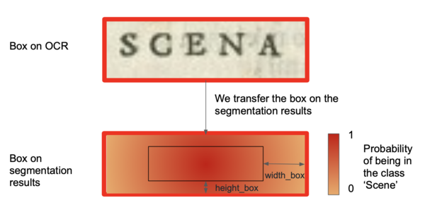
Then, we focus on a word and its particular box. We compute the mean of the class probability of all the pixels figuring in a smaller ratio of the box, which is centered in the true box. We don't read all the pixels of the box as the pixels further away from the center of the box have less chance of being in the class, and because at the end only the center ones matter to now if we need to keep the text in the box or not. This allows us to have a better precision on our results and gain some time.
We then compute the mean value of the corresponding pixels in the OCR result - that, recall, were either 0 or 1. We define a mean_threshold for each attribute which specifies at which point the word in the box is kept as being part of the class. We will only keep these words for our analysis.
After that, we return for each extracted word that matters to us their top left box x and y coordinate, that we got from the OCR results. We first order the words based on their x coordinates and allocate them to 0 if they're in the left page, respectively 1 for the right page. This is done using the defined ranges of the image from which to extract the words for each attribute. Then we order the words based on the y coordinates from top to bottom.
In the end, we have for each page the extracted words and their respective attribute affiliation (name, scene, description) in the order of appearance.
Creating the network of a libretto
From the list of all the ordered attributes of the libretto, we want to create a network that will be used to visualize the relationships between the characters in time. There are many challenges here.
Let's start with the problem of retrieving the names. In the dialogues, there are only abbreviations indicating which character is talking. We would want to find the full name of course. Luckily, in the description just below each scenes, there is a small text describing the place, and which characters play in the scene, by their complete name. We use this fact to find back the full name from the abbreviations.
We proceed the following way : first, with all the abbreviations we found, we create a regular expression pattern, that we will use to match the full name. For example, if we have Ant we will create a pattern An.*t*., and if we have Aut we will get Au.*t*.. We try to match them with words that appeared in the description fields. The pattern means that we look for a word that begins with An followed by zero or many random characters followed by t followed by zero or more random characters. Once we found the full name for every abbreviations, a problem still remains : we might get some variants of the same full name, for example Antigona or Autigona !
Because the OCR might have detected variants of the same name, we need to clean that. We could first think of clustering with K-means for example, but this doesn't work because we don't know a-priori the number of clusters, which corresponds to the number of characters in the libretto. There exists techniques such as K-metroids that could be a possible solution, but we would have to think a bit about how to implement it for strings. Because of time constraints, we choose another approach : similarity distances, and in our case the edit distance from Levenstein. This distance counts the number of edits (deletion, addition, replacement) between two strings, and if it is equal or less than two, we decide that they refer to the same name. For example, Antigona and Autigona would be of a distance of one, and thus grouped together. But then we need to decide which name is the true one. We do that by selecting the one that appears the most often in the whole libretto, assuming that the OCR would be right most of the time.
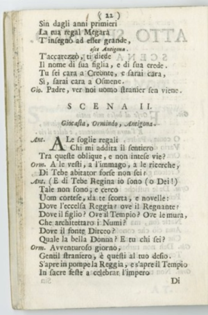
For the scenes, we face another problem. We need a way to correctly count and order them. The acts each start with the SCENA PRIMA, meaning first scene. Then again for every act, the very last scene is SCENA ULTIMA. Moreover, the scenes are counted using roman numbers. Simply extracting the number is complicated for several reasons: first, we would need to find back the index corresponding to the roman number. This could probably be done using a dictionary that maps the values. However, there is a second problem : because the typology of the scenes is very spaced (see figure on the right), the OCR considers sometimes that each letter composing the number is a different word. We then have again one of our first problem: reordering the extracted words correctly based on the scanning orientation.
So we need to find another algorithm to do that. We observe that the OCR detected quite well the SCENA term. We will assume that every time we find a scene tagged SCENA or its variants SCEN or SCENO, we increment the counter of scenes and add a new scene at this place. To find where a new act begins, and thus where to start the counter over, we simply look for an occurence of a scene tagged PRIMA. This will define where an act starts.
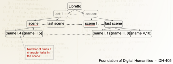
Finally, with all this, we get a tree where we have the acts, scenes, names of characters appearing in the scenes and their number of occurrences in the scene. The tree would look something like this :
Graph Representation of the Network
Now that we have the tree of the libretto, we can build our network visualization.
We create an interractive graph using D3.js. Most of the code comes from here.
We need to tweak a bit our previous tree to format it in the following way :
- A key "nodes" which contains:
- key id, the name of the character
- key act_N: the weight of the node, being the number of times the character appeared in the act N. There are N keys "act", depending of the number of acts figuring in the libretto.
- A key "links" which contains:
- key source, a character name
- key target, another character name
- key act_N: the weight of the link, being the number of scenes where the source and target characters appear together. There are N keys "act", depending of the number of acts figuring in the libretto.
That way, we can visualize the importance of each character and each link between the characters, by looking at the size of the node or link. You can also choose which libretto and acts you want to visualize.
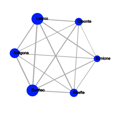
Here is the example of the network of Antigone :
We see that in the whole libretto, all the characters interact together and we can tell which character are more important than others by looking at the size of their nodes and links.
Generalization
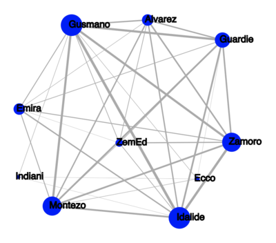
We now try to see how our full pipeline generalizes to other libretti. We choose, arbitrarily, Gli americani libretto.
Here is what we got :
We see that our algorithm works, but is a bit less good than on Antigone. This is mainly because of the hyperparameters that we previously chose to fit best the Antigone libretto. For example, abbreviations were on the images really close to the text, which made us extract words from the dialogue as names. We overfitted on Antigone, which leads to some noise in the final Gli network. For example, 'ZemEd' is not a character is the libretto.
Nevertheless, we have results and more importantly we got a full pipeline that can be very easily re-used for every other libretto, to automatically find the relationships between the characters, and get some more insight about a libretto.
Quality Assesment
First, let's analyse how well the segmentation model worked. Our best model has a mean Intersection Over Union of 0.55. This could have been improved with more training and validation data, and the number is not very high because of the very diverse nature of the libretto. There are as many layouts/formats as different libretto.
It still worked nicely on the Antigone's libretto that we chose :
We also analyse the overall result of our algorithm. To do that, we write by hand the real tree associated to the two libretto we tested on. This will constitute our ground truth. We use the zss algorithm and library, explained in this paper, that computes the edit distance between two trees. The edit distance is the number of modifications we need to perform to transform a tree into another.
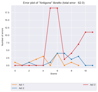
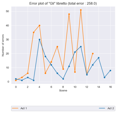
We computed the total edit distance between our extracted tree structure libretto and the ground truth, to get an overall score of how well we did. We also computed per each act the edit distances between our extracted tree structure libretto and the ground truth one. Indeed, we assume that we get a high edit distance whenever our model forgot/added a wrong scene, which will then shift the values of the nodes (i.e. the scene value) in the tree structure by 1 and thus count the children of the tree (being the characters) as being wrong. Therefore this plot will point at the extra added/removed scene. We also plot the error scene by scene.
Let's analyse the results we got.
We see that Antigone has a distance error of 48 and Gli of 258. This is coherent with our first view of the network data. Antigone seemed correct and Gli had more noise into it. We can look more in details at the graphs. For Antigone, we see that there is never a distance greater than 4, except for one big spike in the red act (it is the third one). To understand this, we look at the network and we see that our algorithm missed the 6th scene !
The error plot for Gli has much higher errors, and that is because the segmentation was not very accurate which leads the algorithm to fail to group correctly the names and abbreviations, and mess up the scenes
Conclusions
In conclusion of this project, we managed to read the names and scenes from a digitized libretto. We then arranged the data in a comprehensible and logic way, to finally display it as a network. In the network, we found a way to illustrate the weight of relationships between characters, along with their evolution over time. We therefore achieved our goal to implement a visualization tool for the evolution of characters' relationships in operas. This work was very focused on one specific libretto - Antigona - and does not generalize well, but we believe that improvements can be made that go into that direction.
Further research
We successfully did a first attempt at automatically analyzing the character's relationships in a libretto, from digitized images of it. However, it is far from being perfect. Here are a few ideas that may move the project forward:
- Improve the segmentation model. We saw that the segmentation model was not performing extremely well because of the large range of different libretti' formats. To make it better, we should train it on more images which need to be more diverse. This would improve its accuracy and as a consequence the one of the whole algorithm.
- Optimizing the hyperparameters automatically. We only did this manually, and we now have a way to measure how well our algorithm did at producing the graph. We could minimize this error over more libretti with respect to the hyperparameters by performing a grid-search on these values. This would allow even better generalization.
- Creating our own distance metric between two libretti's tree. We are using a general algorithm that compares two trees. It could be nice to have a metric that reflects actually how we want to penalize forgetting an act, a scene, a character, ...
Links
Planning
| Week | To do |
|---|---|
| 12.11. (week 9) | Step 1: Segmentation model training, fine tuning & testing |
| 19.11. (week 10) | Step 2: Information extraction & cleaning |
| 26.11. (week 11) | Finishing Step 2 |
| 03.12. (week 12) | Step 3: Information storing & network visualization |
| 10.12. (week 13) | Finishing Step 3 and Finalize Report and Wikipage (Step 4: Generalization) |
| 17.12. (week 14) | Final Presentation |
Step 1
- Train model on diverse random images of Rolandi’s libretti collection (better for generalization aspects)
- Test model on diverse random images of Rolandi’s libretti collection
- Test on a single chosen libretto:
- If bad results, train the model on more images coming from the libretto
- If still bad results (and ok with the planning), try to help the model by pre-processing the images beforehand : i.e. black and white images (filter that accentuates shades of black)
- Choose a well-formatted and not too damaged libretto (to be able to do step 2)
Step 2
- Extract essential information from the libretto with OCR
- names, scenes and descriptions
- if bad results, apply pre-processing to make the handwriting sharper for reading
- If OCR extracts variants of same name:
- perform clustering to give it a common name
- apply distance measuring techniques
- find the real name (not just the abbreviation) of the character using the introduction at the start of the scene
Step 3
For one libretto:
- Extract the information below and store it in a tree format (json file):
- Assessment of extraction and cleaning results
- Create the relationship network:
- nodes = characters’ name
- links = interactions
- weight of the links = importance of a relationship
- weight of nodes = speech weight of a character + normalization so that all the scenes have the same weight/importance
Step 4: Optionnal
- See how our network algorithm generalizes (according to the success of step 1) to five Rolandi’s libretti.
- If this does not generalize well, strengthen our deep learning model with more images coming from these libretti.
