Austrian cadastral map: Difference between revisions
| (One intermediate revision by the same user not shown) | |||
| Line 110: | Line 110: | ||
=== Evaluation === | === Evaluation === | ||
To evaluate our models, we | To evaluate our models, we created more masks to be used as tests. We then compared the geometries resulting from the segmentation pipeline on the cadaster image with the corresponding mask. | ||
To compare our results to what was expected, we first need to transform our hand-made mask to polygons so that they are comparable. For that goal, we use the same method as the post-processing (watershed) to detect geometries. | To compare our results to what was expected, we first need to transform our hand-made mask to polygons so that they are comparable. For that goal, we use the same method as the post-processing (watershed) to detect geometries. | ||
| Line 123: | Line 123: | ||
* one trained on the 1808 cadaster (<code>model_edges3_1808</code>) | * one trained on the 1808 cadaster (<code>model_edges3_1808</code>) | ||
* two trained on the Austrian cadaster with different patience for early stopping (<code>model_edges2_n01</code> and <code>model_edges2_n02</code>) | * two trained on the Austrian cadaster with different patience for early stopping (<code>model_edges2_n01</code> and <code>model_edges2_n02</code>) | ||
* one trained on the Austrian cadaster after | * one trained on the Austrian cadaster after creating two extra masks (<code>model_edges2_n03</code>) | ||
and three different class models, all trained on the Austrian cadaster: | and three different class models, all trained on the Austrian cadaster: | ||
* one with "background" in white (<code>model_classes_n01</code>) | * one with "background" in white (<code>model_classes_n01</code>) | ||
* one without differentiating water and streets (<code>model_classes_nowater_n01</code>) | * one without differentiating water and streets (<code>model_classes_nowater_n01</code>) | ||
* one with "background" in black (<code>model_classes_inv_n01</code>) | * one with "background" in black after creating two extra masks (<code>model_classes_inv_n01</code>) | ||
We tested all 12 combinations on two images and found that we got the best results using <code>model_edges2_n01 and n02</code> and <code>model_classes_inv_n01</code>. | We tested all 12 combinations on two images and found that we got the best results using <code>model_edges2_n01 and n02</code> and <code>model_classes_inv_n01</code>. | ||
Latest revision as of 17:11, 15 December 2020
Abstract
Many Venetian maps and cadasters were digitized in the Venice Time Machine project. Cadastral maps offer a detailed representation of properties in a specific area. As a part of the Time Machine, a pipeline was created to extract geometries from the 1808 Napoleonian cadastral map of Venice. The goal of this project is to use this pipeline to extract geometries from the 1848 Austrian cadaster and adapt it as necessary. The extracted geometries could then be used to compare the different shapes of the city of Venice in 1808, 1848 and eventually today.
Planning
Project steps
1. First overview
- Install the pipeline used on the 1808 cadaster and train a few models on it (done)
- Use the models trained to predict geometries on the Austrian cadaster (done)
2. Training on the Austrian cadaster
- Georeference the Austrian cadaster
- Prepare training data from the Austrian cadaster (make masks)
- Adapt model to the Austrian cadaster
- Train models on the prepared data
- Evaluate models
3. Optimizing of post-processing
- Understand the post-processing done on the probability maps
- Research similar solutions
- Try to optimize post-processing
4. Extensions (if time)
- Compare new 1848 geometries to 1808 ones
- Make some statistics on the similarities/differences
Timetable
| Timeframe | Model | Post-processing |
|---|---|---|
| Weeks 8-10 | Finish georeferencing | Examine post-processing |
| Week 10-11 | Prepare training data from Austrian cadaster, adapt model | |
| Weeks 11-13 | Train and test models on Austrian cadaster | Research and optimize post-processing |
| Week 13 | Combine and evaluate results | If time, compare with 1808 geometries |
| Week 14 | Final Project presentation |
Methods
Georeferencing
While working with maps and cadaster, an important task is the georeferencing of the images. Indeed, the geometries resulting from processing of the digitized cadastral map have to be comparable to others and placed correctly on a world map. To achieve this, the original cadaster images are georeferenced using QGIS, a geographic information system application. Common points between the image and a current map, such as OpenStreet Map, are identified and used by the georeferencement tool of QGIS to create a georeferenced tif document. This ensures that the geometries created from this document can be placed correctly on a world map.
DHSegment-torch
Overview
Historical document segmentation has been an issue in Digital Humanities for a number of years, due to the diversity of these documents. DHSegment is a method that uses a generic CNN-architecture that can be used for multiple different processing tasks.
This method consists of two steps. The first step takes the images the type of documents to be processed and the masks associated as input to train a Fully Convolutional Neural Network. When given a new image corresponding to the same type of document, the network will output a map of label probabilities associated with each pixel. The second step is post-processing. It takes the probabilities map and using standard image processing techniques, transforms it to an output depending on the task.
Adaptation
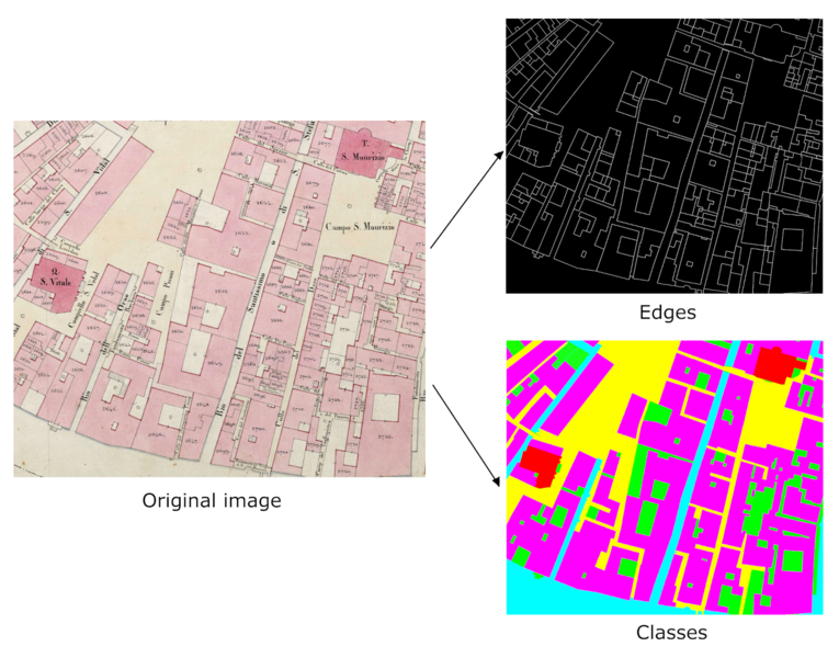
In our project, we had to adapt the DHSegment-torch methods used on the 1808 cadaster to the 1848 one. Reusing the exact models was not conclusive as colour conventions were not the same between the cadasters. We had to make new masks ourselves on the 1848 cadaster images using GIMP. The masks use colours corresponding to the class labels that we wanted the model to recognise; edge, street, water, courtyard, building and church, see Fig. 1. These masks and the associated images were then given to the network to train different models. One model was trained to recognise only the edges, another only the classes and the last could recognise both.
Post-processing
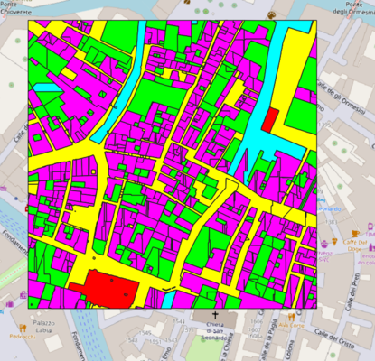
The same post-processing as for the 1808 cadaster was used on the probabilities maps given as outputs of our models. First, a watershed is done using the local minima taken from the predicted edge map as markers. Then, cv2.findContours, a function often used to find the shapes in image processing, is used to create the geometries from the watershed. The geometries are assigned the majoritarian class and transformed into a GeoJSON file that can be opened in QGIS. Fig. 2 shows an example of geometries extracted on a sample image and opened in QGIS.
Motivation and implementation
DHSegment is now widely used for very diverse historical documents segmentation tasks. The goal of this project was to assess if the DHSegment pipeline used to extract geometries from the 1808 Napoleonian cadaster could be reused for other cadasters using different standards.
To test this, the 1848 Austrian cadastral map was used. After training models on the existing images and masks from the 1808 cadaster, we tested them on samples from the 1848 cadaster.
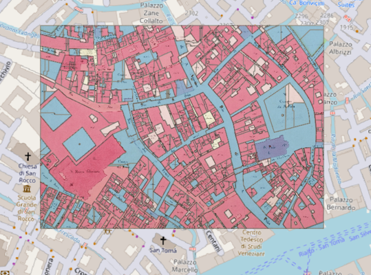
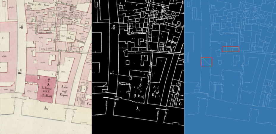
Unfortunately, we quickly found out that the differences in standards made it hard for the model to differentiate classes on the 1848 images, especially between water, street and courtyards, see Fig. 3. We then decided to train a different model with masks from the 1848 cadaster directly. We made six different masks from diverse parts of the cadaster. We also then used different classes in our new model, allowing it to also classify churches, which were not differentiated in the 1808 cadaster. Surprisingly, the new model was also able to find water despite it looking very similar to courtyards on the 1848 cadaster. Edge detection was already pretty good with the models trained on the 1808 cadaster so we focused also on the post-processing to see if we could improve it some way.
Results and evaluation
Results
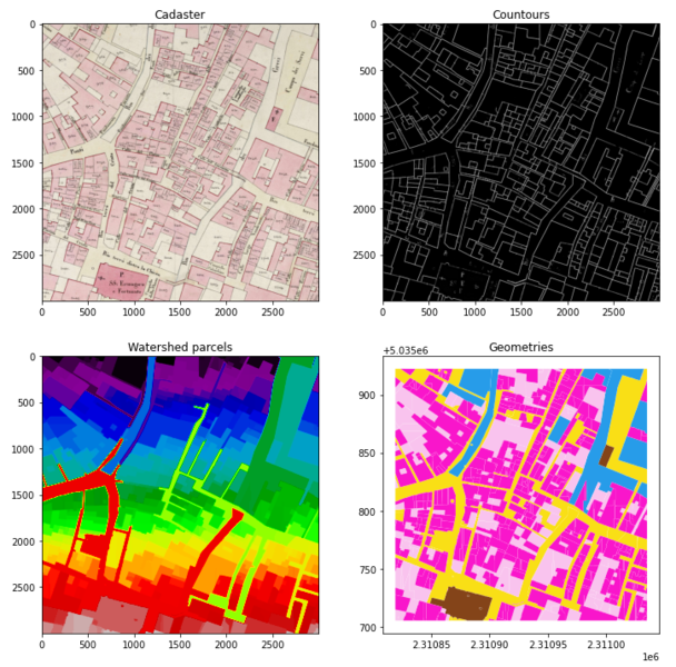
The first models trained on the 1848 cadaster were not very convincing so we made more masks and changed some parameters on the models. We found that while the probabilities maps for edges looked almost perfect, the watershed added or removed many geometries, as can be seen on the 'Geometries' of Fig. 4. To try and fix that, we manually implemented a function that took the contours taken from the edges probability maps and tried to smooth them by filling the small existing gaps on linear edges. The function works but take way too long on even small images, so we decided to look for alternatives to detect lines and holes in them. We started looking at OpenCV tools like using goodFeaturesToTrack to detect holes and filling them using dilate and erode with a linear kernel but unfortunately, we did not have enough time to finish implementing it.
Evaluation
To evaluate our models, we created more masks to be used as tests. We then compared the geometries resulting from the segmentation pipeline on the cadaster image with the corresponding mask.
To compare our results to what was expected, we first need to transform our hand-made mask to polygons so that they are comparable. For that goal, we use the same method as the post-processing (watershed) to detect geometries. Once that is done, we compute the union of all polygons for each class for both the predicted geometries and the mask (real) geometries to obtain a geometry collection per class. With this, we compute the intersection and union between real and predicted geometries to compute the IOU per class – that is the ratio of the intersection's area over the union's area. From these, we compute the mean IOU as well as a weighted average of the IOU, with the weight of each class corresponding to the area of each class in the mask.
For the edges, we consider all points with probability greater than 0.1 (the value used for the prediction watershed) to be part of an edge. We use this approximation because we do not actually obtain geometries for edges, though this could likely be improved by detecting polygon boundaries from the classes. We then compute the IOU by comparing the arrays containing the edges as binary values (1 if an edge is detected, 0 otherwise) and divide the number of ones common to both arrays (intersection area) by the number of ones present in either array (union area). We also compute the ratio of correctly detected edges as the area of the intersection divided by the area of the edges from the mask. One limit of this approximation is that we do not account for edges "invented" by using the watershed algorithms in our post-processing, which we can qualitatively see on Figure 5.
We tested four different edge models:
- one trained on the 1808 cadaster (
model_edges3_1808) - two trained on the Austrian cadaster with different patience for early stopping (
model_edges2_n01andmodel_edges2_n02) - one trained on the Austrian cadaster after creating two extra masks (
model_edges2_n03)
and three different class models, all trained on the Austrian cadaster:
- one with "background" in white (
model_classes_n01) - one without differentiating water and streets (
model_classes_nowater_n01) - one with "background" in black after creating two extra masks (
model_classes_inv_n01)
We tested all 12 combinations on two images and found that we got the best results using model_edges2_n01 and n02 and model_classes_inv_n01.
Deliverables
Our deliverables consist of a folder containing all data from the 1848 cadaster used for the training our models and the Jupyter Notebook used for testing and geometries extraction. The training folder contains cropped images from the Austrian cadastral map and the corresponding masks, edges only, classes only and both. It contains also the txt files for the edge and classes colors and the csv files giving the path to the training images on the iccluster server. These are linked via the config files containing the parameters of the models. The Notebook is taken from the 1808 pipeline and adapted to our model.
The deliverables can be found on : https://github.com/EvaLaini/fdh_austrian_cadaster_extraction
