Switzerland Road extraction from historical maps: Difference between revisions
| (59 intermediate revisions by 2 users not shown) | |||
| Line 6: | Line 6: | ||
== Motivation == | == Motivation == | ||
Historical maps contain rich information, which | Historical maps contain rich information, which is helpful in urban planning, historical study, and various humanities research. Digitization of massive printed documents is a significant step before further research. However, most historical maps are scanned in rasterized graphical images. To conveniently use geographic data extracted from these maps in GIS software, vectorization is needed. | ||
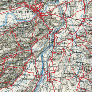
However, vectorization process has always been a challenge due to manual painting. In this project, we try to use dh-segmentation tool for automatic vectorization. With 60 high-resolution patches(5km*5km) for the training dataset, the model is tested on randomly selected patches and proposed to approximate | However, the vectorization process has always been a challenge due to manual painting. In this project, we try to use the dh-segmentation tool for automatic vectorization. With 60 high-resolution patches(5km*5km) for the training dataset, the model is tested on randomly selected patches and proposed to approximate idealised main roads of the Dufour map of the selected region -- Solothurn in Switzerland. | ||
==Description of the Deliverables== | |||
Github repository '''[https://github.com/YinghuiJiang/Switzerland-Road-extraction-from-historical-maps]''' with all materials necessary to demonstrate the results of applying the dhSegment to road extraction from historical maps, vectorization, skeletonization and georeferencing: | |||
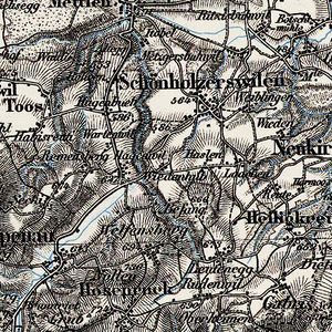
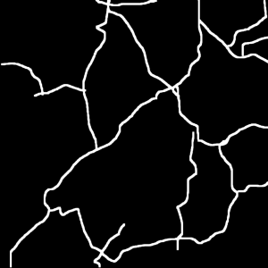
* data - folder with input data for the dhSegment tool, it contains 2 folders: 'images' (contains 60 jpeg patches from different parts of the Dufour map 1000 by 1000 pixels) and 'labels' (contains 60 png binary labels with road annotations for the mentioned patches). Images from this folder were used as a training dataset for dhSegment. | |||
* images_predict - folder with 9 overlapping patches of the Dufour map. These patches represent a small region of Switzerland containing Solothurn. This region was not presented in the training dataset. | |||
*img - folder that contains the results of road segmentation, skeletonization, vectorization and georeferencing for the selected testing dataset: | |||
1) original_tiff_patch - folder with 9 original tiff patches downloaded from GeoVITe. They contain information about the geographic coordinates. | |||
2) Final_line.dbf - one of the automatically generated files. | |||
3) Final_line.points - file with Ground Control Points. | |||
4) Final_line.shp - the final result of the vectorization: the vectorized historical map of Solothurn region | |||
5) Final_line.shx - one of the automatically generated files. | |||
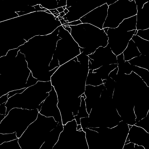
6) Full_image.png - predictions of roads for the region combined from 9 testing patches (Solothurn). | |||
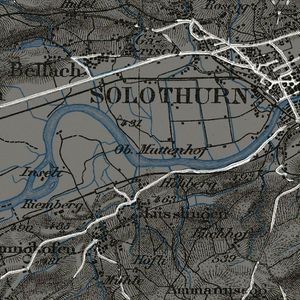
7) Full_map_pred.png - predictions of roads highlighted in the original map of the region. | |||
8) georeferenced_sk.tif - georeferenced vecorized map of predicted roads. | |||
9) sk_Full_image.png - result after skeletonization of the Full_image.png. | |||
Notebooks containing the main coding parts: | |||
* dhSegment.ipynb.zip - compressed jupyter notebook with the results of road segmentation for images_predict. The code was taken from this repository: https://github.com/dhlab-epfl/dhSegment-torch and modified for the purpose of this project. You will find all additional necessary files in the mentioned repository. For additional instructions about the model please refer to https://dhsegment.readthedocs.io/en/latest/index.html. | |||
* skeletonization.ipynb - jupyter notebook with code for skeletonization. | |||
* vectorization.ipynb - jupyter notebook with code for vectorization. | |||
== Plan and Milestones == | == Plan and Milestones == | ||
| Line 22: | Line 51: | ||
'''Milestone 3:''' | '''Milestone 3:''' | ||
* Download the final dataset automatically using the python script: patches with corresponding coordinates completely covering | * Download the final dataset automatically using the python script: patches with corresponding coordinates completely covering the selected region of Switzerland. | ||
* Test the dhSegment tool on the final dataset. | * Test the dhSegment tool on the final dataset. | ||
'''Milestone 4:''' | '''Milestone 4:''' | ||
* Get the vectorised map of roads with skeletonization in Python using OpenCV. | * Get the vectorised map of roads with skeletonization in Python using OpenCV. | ||
* | * Prepare a final presentation. | ||
{| class="wikitable" | {| class="wikitable" | ||
| Line 59: | Line 88: | ||
*Test the pre-trained model provided by DHLAB on the created small dataset | *Test the pre-trained model provided by DHLAB on the created small dataset | ||
*Improve and modify the algorithm of the segmentation tool | *Improve and modify the algorithm of the segmentation tool | ||
| align="center" | | | align="center" | ✓ | ||
|- | |- | ||
| By Week 12 | | By Week 12 | ||
| | | | ||
*Download all patches automatically with the prepared python script and create the main dataset covering | *Download all patches automatically with the prepared python script and create the main dataset covering different regions of Switzerland | ||
*Work on road extraction for | *Work on road extraction for different regions: apply the segmentation process to the main dataset | ||
*Finish Georeferencing and finalize the vectorised map | *Finish Georeferencing and finalize the vectorised map | ||
| align="center" | | | align="center" | ✓ | ||
|- | |- | ||
| By Week 14 | | By Week 14 | ||
| | | | ||
*Sort out all the data in the Github repository | *Sort out all the data in the Github repository | ||
*Finish the Wiki page and prepare for the final presentation | *Finish the Wiki page and prepare for the final presentation | ||
| align="center" | | | align="center" | ✓ | ||
|} | |} | ||
| Line 81: | Line 109: | ||
*The 1:100 000 Topographic Map of Switzerland was the first official series of maps that encompassed the whole of Switzerland. It was published in the period from 1845 to 1865 and thus coincides with the creation of the modern Swiss Confederation. | *The 1:100 000 Topographic Map of Switzerland was the first official series of maps that encompassed the whole of Switzerland. It was published in the period from 1845 to 1865 and thus coincides with the creation of the modern Swiss Confederation. | ||
*Classification : | *Classification: Our goal was to demonstrate segmentation of the main roads in the historical map. We decided to select only roads bounded by solid lines on both sides. That's why, we didn't annotate paths, railway tracks and rivers in the stage of creating labels. | ||
*Layer: Topographic Raster Maps - Historical Maps - Dufour Maps | *Layer in GeoVITe: Topographic Raster Maps - Historical Maps - Dufour Maps | ||
*Coordinate system: CH1903/LV03 | *Coordinate system in GeoVITe: CH1903/LV03 | ||
*Predefined | *Predefined Grid in GeoVITe: 1:25000 | ||
*Patch Size: 1000 by 1000 pixels | *Patch Size: 1000 by 1000 pixels | ||
*Region selected for testing: 1127: Solothurn (name and number of the region are taken from GeoVITe) | |||
'''DhSegment:''' | '''DhSegment:''' | ||
| Line 97: | Line 127: | ||
'''Data preparation:''' | '''Data preparation:''' | ||
* | This stage took a lot of time because in the beginning we didn't have any dataset with original patches of the Dufour map. We tried different approaches of collecting data and here we want to tell a little bit about them. | ||
* Downloading data from Swisstopo: journey through time. Our first idea was to download patches automatically using a python script. This script collected small parts of the map directly from the web-page using their URLs. The main problem was that only a grayscale version of the map was available in Swisstopo. The resolution of the resulting patches was quite small. While annotating them, we faced the problem of distinguishing roads from rivers in these patches. That was the main reason why we decided to abandon this approach and try another one. | |||
* | * Downloading data from GeoVITe. We started with trying to apply the same python script for downloading data to GeoVITe, but it wasn't successful. The maps in GeoVITe are stored differently and we couldn't find a way to download them automatically. That's why, we decided to focus on a small region of Switzerland instead of testing our model on the whole Dufour map. The solution was to use the GeoVITe's user interface for downloading small parts of the map. Finally, we manually downloaded 60 patches from different parts of Switzerland and named them using the stated rule: {number_of_the_patch}_{number_of_the_region_in_GeoVITe}.tiff, where number_of_the_patch was in a range [1, 60] and number_of_the_region_in_GeoVITe was the number of the selected region in GeoVITe's grid. We almost always took the right upper corner of the select region. This system helped us to avoid overlapping of the training patches. For the testing dataset we downloaded 9 overlapping patches corresponding to the GeoVITe's region 1127: Solothurn. The overlapping patches were chosen because dhSegment usually gives worse results for the edge regions of the processed image. | ||
'''Labeling:''' | '''Labeling:''' | ||
| Line 114: | Line 146: | ||
|[[File:17 1074label.png|thumb|center|300px|Figure3:label of the sample patch]] | |[[File:17 1074label.png|thumb|center|300px|Figure3:label of the sample patch]] | ||
|} | |} | ||
== | '''dhSegment:''' | ||
The main limitation of our project is due to the data source platform. GeoVITE only allows small patches downloading, while automatic downloading from other sources leads to unsatisfying low-quality images. | |||
The code from this GitHub repository https://github.com/dhlab-epfl/dhSegment-torch was used and modified for the purpose of road segmentation. In the corresponding Jupiter Notebook in our GitHub repository you can find data, all modified coding parts necessary to perform road segmentation and the obtained results. | |||
'''OpenCV:''' | |||
OpenCV is used for skeletonization to reduce foreground regions in the binary image that largely preserves the extent and connectivity of the original region while throwing away most of the original foreground pixels. It facilitates quick and accurate image processing on the light skeleton instead of an otherwise large and memory-intensive operation on the original image. | |||
typically 1 pixel | |||
two basic morphological operations: dilation and erosion | |||
First, it starts off with an empty skeleton. Then, the opening of the original image is computed. After that, the opening is subtracted from the original image. Afterward, the union of the current skeleton and temp are computed to erode the original image and refine the skeleton. Finally, Repeat the steps above until the original image is completely eroded. | |||
'''GDAL:''' | |||
It's used for processing raster and vector geospatial data. As a library, it presents a single raster abstract data model and single vector abstract data model to the calling application for all supported formats. It's mainly for vectorization in our project. | |||
'''QGIS:''' | |||
QGIS is an open-source Geographic Information System. It's used for georeferencing in our project. We used ground control points ( four corners' coordinates) for georeferencing. | |||
== Discussion of Limitations == | |||
* The main limitation of our project is due to the data source platform. GeoVITE only allows small patches downloading, while automatic downloading from other sources leads to unsatisfying low-quality images. Thus, we only focused on the selected region in Switzerland. | |||
* Not all roads were identified by the neural network. And the additional training of the model didn't help to improve the results. This problem is caused by the limitation of the training dataset: 60 chosen patches are not enough to represent the variety of different landscapes present in the Dufour map. For example, look at the map with predicted roads below: the majority of roads were annotated correctly, however, at the bottom right of the image there are some areas with missed roads. One of the possible reasons is that there were not enough patches showing roads in the bush area or next to the large amount of buildings in the training dataset. | |||
{|class="wikitable" style="margin: 1em auto 1em auto;" | |||
|- | |||
|[[File:Missing.jpg|thumb|center|300px|Figure: Testing patch with missed roads]] | |||
|} | |||
== Results == | == Results == | ||
== | |||
* Our most important result is that we achieved the goal of the project: now we are able to present the vectorisation of the historical road map of a small region in Switzerland. And the same result can be obtained for the whole Dufour map, if all the data is available and more different patches are added to the training dataset. | |||
* We proved that dhSegment tool can be used for the purpose of road segmentation and that the results are more than satisfactory. | |||
* We implemented skeletonization and vectorisation of the obtained map with predicted roads. | |||
* Some of the roads were missed during the process of predicting. We tried to change the threshold for the probability map, but in the resulting image the roads were thicker and additional noise appeared. That's why, we demonstrate the results obtained this way in the Jupyter notebook, however, we don't use them. | |||
* In the images below you can find a binary map with predicted roads for the Solothurn region, its skeletonized version, corresponding original region with highlighted maps and the results of vectorization. | |||
{|class="wikitable" style="margin: 1em auto 1em auto;" | |||
|- | |||
|[[File:Full_image.png|thumb|center|300px|Figure 4: Image after training( target region)]] | |||
|[[File:Skeletonized_img.png|thumb|center|300px|Figure 5: Image after skeletonization( target region)]] | |||
|} | |||
{|class="wikitable" style="margin: 1em auto 1em auto;" | |||
|- | |||
|[[File:Map predictions.jpg|thumb|center|300px|Figure 6: Map with highlighted predictions]] | |||
|[[File:Original.jpg|thumb|center|300px|Figure 7: Original map (target region)]] | |||
|} | |||
{|class="wikitable" style="margin: 1em auto 1em auto;" | |||
|- | |||
|[[File:shp.png|thumb|center|300px|Figure 8: Vectorised image with extracted roads( target region)]] | |||
|[[File:line_img.png|thumb|center|300px|Figure 9: Comparison with orignal map( target region)]] | |||
|} | |||
== Links == | == Links == | ||
*Github repository: '''[https://github.com/YinghuiJiang/Switzerland- | *Github repository: '''[https://github.com/YinghuiJiang/Switzerland-Road-extraction-from-historical-maps]''' | ||
*GeoVITE :'''[https://geovite.ethz.ch/]''' | *GeoVITE :'''[https://geovite.ethz.ch/]''' | ||
*dhSegment:'''[https://github.com/dhlab-epfl/dhSegment]''' | *dhSegment:'''[https://github.com/dhlab-epfl/dhSegment]''' | ||
Latest revision as of 16:00, 22 December 2021
Introduction
Historical maps provide valuable information about spatial transformation of the landscape over time spans. This project, based on historical maps of Switzerland, is to vectorize road network and landcover and to visualize the transformation using a machine vision library developed at the DHLAB.
The main data source of this project is GeoVITe (Geodata Versatile Information Transfer environment),a browser-based access to geodata for research and teaching, operated by the Institute of Cartography and Geoinformation of ETH Zurich (IKG) since 2008.
Motivation
Historical maps contain rich information, which is helpful in urban planning, historical study, and various humanities research. Digitization of massive printed documents is a significant step before further research. However, most historical maps are scanned in rasterized graphical images. To conveniently use geographic data extracted from these maps in GIS software, vectorization is needed.
However, the vectorization process has always been a challenge due to manual painting. In this project, we try to use the dh-segmentation tool for automatic vectorization. With 60 high-resolution patches(5km*5km) for the training dataset, the model is tested on randomly selected patches and proposed to approximate idealised main roads of the Dufour map of the selected region -- Solothurn in Switzerland.
Description of the Deliverables
Github repository [1] with all materials necessary to demonstrate the results of applying the dhSegment to road extraction from historical maps, vectorization, skeletonization and georeferencing:
- data - folder with input data for the dhSegment tool, it contains 2 folders: 'images' (contains 60 jpeg patches from different parts of the Dufour map 1000 by 1000 pixels) and 'labels' (contains 60 png binary labels with road annotations for the mentioned patches). Images from this folder were used as a training dataset for dhSegment.
- images_predict - folder with 9 overlapping patches of the Dufour map. These patches represent a small region of Switzerland containing Solothurn. This region was not presented in the training dataset.
- img - folder that contains the results of road segmentation, skeletonization, vectorization and georeferencing for the selected testing dataset:
1) original_tiff_patch - folder with 9 original tiff patches downloaded from GeoVITe. They contain information about the geographic coordinates.
2) Final_line.dbf - one of the automatically generated files.
3) Final_line.points - file with Ground Control Points.
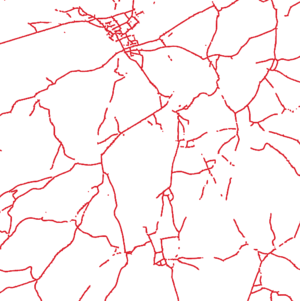
4) Final_line.shp - the final result of the vectorization: the vectorized historical map of Solothurn region
5) Final_line.shx - one of the automatically generated files.
6) Full_image.png - predictions of roads for the region combined from 9 testing patches (Solothurn).
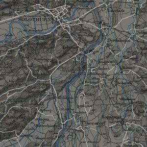
7) Full_map_pred.png - predictions of roads highlighted in the original map of the region.
8) georeferenced_sk.tif - georeferenced vecorized map of predicted roads.
9) sk_Full_image.png - result after skeletonization of the Full_image.png.
Notebooks containing the main coding parts:
- dhSegment.ipynb.zip - compressed jupyter notebook with the results of road segmentation for images_predict. The code was taken from this repository: https://github.com/dhlab-epfl/dhSegment-torch and modified for the purpose of this project. You will find all additional necessary files in the mentioned repository. For additional instructions about the model please refer to https://dhsegment.readthedocs.io/en/latest/index.html.
- skeletonization.ipynb - jupyter notebook with code for skeletonization.
- vectorization.ipynb - jupyter notebook with code for vectorization.
Plan and Milestones
Milestone 1:
- Choose the topic for the project, present the first ideas. Get familiar with the data provided.
- Define the final subject of the project. Find reliable sources of information. Get familiar with the dhSegment tool.
Milestone 2: (Now)
- Prepare a small dataset (60 samples) for training and testing with Convolutional Neural Network, main part of the dhSegment tool. This dataset should consist of small patches extracted from the Dufour Map of Switzerland, their versions in jpeg format and binary labels created in GIMP.
- Determine the way of downloading a huge amount of samples from GeoVITe.
- Prepare for the mid-term presentation and write the project plan and milestone.
- Try the dhSegment tool with the created dataset. Evaluate the results, modify the algorithm. Make conclusions about using this tool for road extraction, advantages and disadvantages of this approach.
Milestone 3:
- Download the final dataset automatically using the python script: patches with corresponding coordinates completely covering the selected region of Switzerland.
- Test the dhSegment tool on the final dataset.
Milestone 4:
- Get the vectorised map of roads with skeletonization in Python using OpenCV.
- Prepare a final presentation.
| Deadline | Task | Completion |
|---|---|---|
| By Week 4 |
|
✓ |
| By Week 6 |
|
✓ |
| By Week 8 |
|
✓ |
| By Week 10 |
|
✓ |
| By Week 12 |
|
✓ |
| By Week 14 |
|
✓ |
Methodology
Dataset:
- Dufour Map from GeoVITe
- The 1:100 000 Topographic Map of Switzerland was the first official series of maps that encompassed the whole of Switzerland. It was published in the period from 1845 to 1865 and thus coincides with the creation of the modern Swiss Confederation.
- Classification: Our goal was to demonstrate segmentation of the main roads in the historical map. We decided to select only roads bounded by solid lines on both sides. That's why, we didn't annotate paths, railway tracks and rivers in the stage of creating labels.
- Layer in GeoVITe: Topographic Raster Maps - Historical Maps - Dufour Maps
- Coordinate system in GeoVITe: CH1903/LV03
- Predefined Grid in GeoVITe: 1:25000
- Patch Size: 1000 by 1000 pixels
- Region selected for testing: 1127: Solothurn (name and number of the region are taken from GeoVITe)
DhSegment:
A generic framework for historical document processing using Deep learning approach, created by Benoit Seguin and Sofia Ares Oliveira at DHLAB, EPFL.
Data preparation:
This stage took a lot of time because in the beginning we didn't have any dataset with original patches of the Dufour map. We tried different approaches of collecting data and here we want to tell a little bit about them.
- Downloading data from Swisstopo: journey through time. Our first idea was to download patches automatically using a python script. This script collected small parts of the map directly from the web-page using their URLs. The main problem was that only a grayscale version of the map was available in Swisstopo. The resolution of the resulting patches was quite small. While annotating them, we faced the problem of distinguishing roads from rivers in these patches. That was the main reason why we decided to abandon this approach and try another one.
- Downloading data from GeoVITe. We started with trying to apply the same python script for downloading data to GeoVITe, but it wasn't successful. The maps in GeoVITe are stored differently and we couldn't find a way to download them automatically. That's why, we decided to focus on a small region of Switzerland instead of testing our model on the whole Dufour map. The solution was to use the GeoVITe's user interface for downloading small parts of the map. Finally, we manually downloaded 60 patches from different parts of Switzerland and named them using the stated rule: {number_of_the_patch}_{number_of_the_region_in_GeoVITe}.tiff, where number_of_the_patch was in a range [1, 60] and number_of_the_region_in_GeoVITe was the number of the selected region in GeoVITe's grid. We almost always took the right upper corner of the select region. This system helped us to avoid overlapping of the training patches. For the testing dataset we downloaded 9 overlapping patches corresponding to the GeoVITe's region 1127: Solothurn. The overlapping patches were chosen because dhSegment usually gives worse results for the edge regions of the processed image.
Labeling:
60 patches (1000x1000 pixels) using GIMP for model testing:
- Original patches with spatial information: tiff
- Patches for training: jpeg
- labels in black and white: png
dhSegment:
The code from this GitHub repository https://github.com/dhlab-epfl/dhSegment-torch was used and modified for the purpose of road segmentation. In the corresponding Jupiter Notebook in our GitHub repository you can find data, all modified coding parts necessary to perform road segmentation and the obtained results.
OpenCV:
OpenCV is used for skeletonization to reduce foreground regions in the binary image that largely preserves the extent and connectivity of the original region while throwing away most of the original foreground pixels. It facilitates quick and accurate image processing on the light skeleton instead of an otherwise large and memory-intensive operation on the original image. typically 1 pixel two basic morphological operations: dilation and erosion First, it starts off with an empty skeleton. Then, the opening of the original image is computed. After that, the opening is subtracted from the original image. Afterward, the union of the current skeleton and temp are computed to erode the original image and refine the skeleton. Finally, Repeat the steps above until the original image is completely eroded.
GDAL:
It's used for processing raster and vector geospatial data. As a library, it presents a single raster abstract data model and single vector abstract data model to the calling application for all supported formats. It's mainly for vectorization in our project.
QGIS:
QGIS is an open-source Geographic Information System. It's used for georeferencing in our project. We used ground control points ( four corners' coordinates) for georeferencing.
Discussion of Limitations
- The main limitation of our project is due to the data source platform. GeoVITE only allows small patches downloading, while automatic downloading from other sources leads to unsatisfying low-quality images. Thus, we only focused on the selected region in Switzerland.
- Not all roads were identified by the neural network. And the additional training of the model didn't help to improve the results. This problem is caused by the limitation of the training dataset: 60 chosen patches are not enough to represent the variety of different landscapes present in the Dufour map. For example, look at the map with predicted roads below: the majority of roads were annotated correctly, however, at the bottom right of the image there are some areas with missed roads. One of the possible reasons is that there were not enough patches showing roads in the bush area or next to the large amount of buildings in the training dataset.
Results
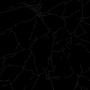
- Our most important result is that we achieved the goal of the project: now we are able to present the vectorisation of the historical road map of a small region in Switzerland. And the same result can be obtained for the whole Dufour map, if all the data is available and more different patches are added to the training dataset.
- We proved that dhSegment tool can be used for the purpose of road segmentation and that the results are more than satisfactory.
- We implemented skeletonization and vectorisation of the obtained map with predicted roads.
- Some of the roads were missed during the process of predicting. We tried to change the threshold for the probability map, but in the resulting image the roads were thicker and additional noise appeared. That's why, we demonstrate the results obtained this way in the Jupyter notebook, however, we don't use them.
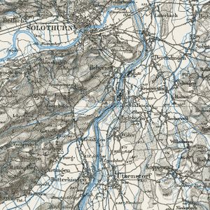
- In the images below you can find a binary map with predicted roads for the Solothurn region, its skeletonized version, corresponding original region with highlighted maps and the results of vectorization.

