Jerusalem 1840-1949 Road Extraction and Alignment: Difference between revisions
Junzhe.tang (talk | contribs) |
Junzhe.tang (talk | contribs) |
||
| (102 intermediate revisions by the same user not shown) | |||
| Line 1: | Line 1: | ||
== | ==Motivation== | ||
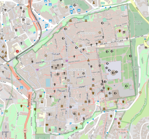
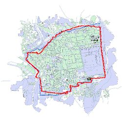
[[File:Osm.png |thumb|Figure 1: Jerusalem In Openstreetmap ]] | |||
[[File: | |||
The creation of large digital databases on urban development is a strategic challenge, which could lead to new discoveries in urban planning, environmental sciences, sociology, economics, and in a considerable number of scientific and social fields. Digital geohistorical data can also be used and valued by cultural institutions. These historical data could also be studied to better understand and optimize the construction of new infrastructures in cities nowadays, and provide humanities scientists with accurate variables that are essential to simulate and analyze urban ecosystems. Now there are many geographic information system platforms that can be directly applied, such as QGIS, ARCGIS, etc. How to digitize and standardize geo-historical data has become the focus of research. We hope to propose a model that can associate geographic historical data with today's digital maps, analyze and study them under the same geographic information platform, same coordinate projection, and the same scale. Eventually, it can eliminate errors caused by scaling, rotation, and the deformation of the map carrier that may exist in historical data and the entire process is automated and efficient. | The creation of large digital databases on urban development is a strategic challenge, which could lead to new discoveries in urban planning, environmental sciences, sociology, economics, and in a considerable number of scientific and social fields. Digital geohistorical data can also be used and valued by cultural institutions. These historical data could also be studied to better understand and optimize the construction of new infrastructures in cities nowadays, and provide humanities scientists with accurate variables that are essential to simulate and analyze urban ecosystems. Now there are many geographic information system platforms that can be directly applied, such as QGIS, ARCGIS, etc. How to digitize and standardize geo-historical data has become the focus of research. We hope to propose a model that can associate geographic historical data with today's digital maps, analyze and study them under the same geographic information platform, same coordinate projection, and the same scale. Eventually, it can eliminate errors caused by scaling, rotation, and the deformation of the map carrier that may exist in historical data and the entire process is automated and efficient. | ||
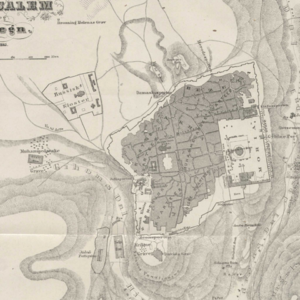
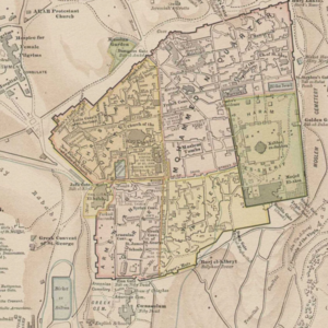
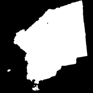
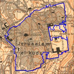
The scale is restricted to Jerusalem in our project. Jerusalem is one of the oldest cities in the world and is considered holy to the three major Abrahamic religions—Judaism, Christianity, and Islam. We did georeferencing among Jerusalem’s historical maps from 1840 to 1949 and the modern map from OpenStreetMap so that the overlaid maps will reveal changes over time and enable map analysis and discovery. We focused on the wall of the Old City as the morphological feature to do georeferencing because the region outside the Old City has seen many new constructions while the Old City has not great changes and the closed polygon of the wall is relatively more consistent than other features like road networks. More specifically, we used dhSegment, a historical document segmentation tool, to extract the wall of the Old City of Jerusalem and proposed an alignment algorithm exploiting the geometrical features of the wall to align the maps. | The scale is restricted to Jerusalem in our project. Jerusalem is one of the oldest cities in the world and is considered holy to the three major Abrahamic religions—Judaism, Christianity, and Islam. We did georeferencing among Jerusalem’s historical maps from 1840 to 1949 and the modern map from OpenStreetMap so that the overlaid maps will reveal changes over time and enable map analysis and discovery. We focused on the wall of the Old City as the morphological feature to do georeferencing because the region outside the Old City has seen many new constructions while the Old City has not great changes and the closed polygon of the wall is relatively more consistent than other features like road networks. More specifically, we used dhSegment, a historical document segmentation tool, to extract the wall of the Old City of Jerusalem and proposed an alignment algorithm exploiting the geometrical features of the wall to align the maps. | ||
==Deliverables== | |||
- The latitudes and longitudes of the four vertices of the raw maps. | |||
- Preprocessed (cropped and resized) patches of the raw maps with images information (including the position of the sub-image in the raw map) stored in a csv file. | |||
- 42 1000 * 1000 annotations of the Old City area. | |||
- Trained segmentation model. | |||
- Code and instructions to reproduce the results on github. | |||
==Methodology== | ==Methodology== | ||
| Line 18: | Line 26: | ||
===Wall Extraction=== | ===Wall Extraction=== | ||
dhSegment is a generic approach for Historical Document Processing | |||
We first used dhSegment to do image segmentation in order to extract the wall polygon from the maps. dhSegment [1] is a generic approach for Historical Document Processing, which relies on a Convolutional Neural Network to predict pixelwise characteristics. The whole process include preprocessing, training, predicting and postprocessing. | |||
[[File:The network architecture is adapted from ResNet-50.jpg|550px|thumb|center|Figure 2: network architecture]] | [[File:The network architecture is adapted from ResNet-50.jpg|550px|thumb|center|Figure 2: network architecture]] | ||
* '''Preprocessing''' | * '''Preprocessing''' | ||
To make the image data fit into the neural networks and to make the old city region more dominant in the image, we cropped and scaled the original image | To make the image data fit into the neural networks and to make the old city region more dominant in the image, we cropped and scaled the original image by hand for subsequent uses. | ||
* '''Map annotating''' | |||
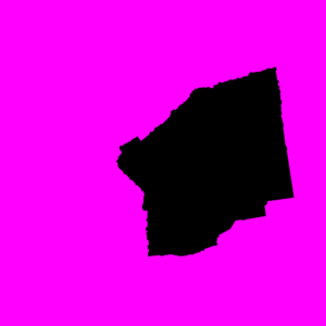
We used Procreate to pixel-wisely label 42 maps according to whether the pixel belong to the old city with different colors (RGB(0, 0, 0) for pixels inside the wall, RGB(255, 0, 255) for pixels outside the wall). | |||
* '''Training''' | * '''Training''' | ||
We divided the 42 annotated patches into 36 and 6 for training and validating respectively, and trained the model with learning rate 5e-5, batch size: 2, N_epochs: 40, and data augmentation like rotation, scaling and color. | |||
{|class="wikitable" style="margin: 1em auto 1em auto;" | {|class="wikitable" style="margin: 1em auto 1em auto;" | ||
| Line 35: | Line 49: | ||
* '''Prediction''' | * '''Prediction''' | ||
By doing prediction on the testing set, we got the predicted old city region and naturally got the contour of it, i.e. the wall. | By doing prediction on the testing set, we got the predicted old city region and naturally got the contour of it, i.e. the wall. | ||
{|class="wikitable" style="margin: 1em auto 1em auto;" | {|class="wikitable" style="margin: 1em auto 1em auto;" | ||
|- | |- | ||
| Line 42: | Line 57: | ||
* '''Postprocessing''' | * '''Postprocessing''' | ||
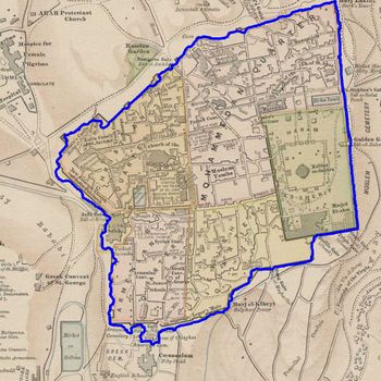
We | We removed the minor noises by retain the largest connected region and drew the contour of it. We put the contour on the original image and find that it generally fits well, although there are some minor deviations. | ||
[[File:1887res contour.jpg|350px|thumb|center|Figure 7: After removing noises and drawing contour]] | [[File:1887res contour.jpg|350px|thumb|center|Figure 7: After removing noises and drawing contour]] | ||
===Wall Alignment=== | ===Wall Alignment=== | ||
After obtaining the wall | After obtaining the wall polygons, we try to fit them to the the reference wall polygon from the OpenStreetMap and obtain the coordinates of the source polygon as well as the four vertices of the source image in the coordinate system of the reference image. | ||
* '''Overview''' | |||
The overall algorithm proposed is shown as follows. We do scaling, transformation and rotation iteratively for a given iteration numbers in order to get a better alignment result since the initial scaling isn't the accurate enough with the angle difference of the source polygon and reference polygon. | |||
:For '''''i = 0''''' to '''''iters ''''': | |||
::Estimate and do scaling | |||
::For each point pair ''''' P ''''' in selected point pair set: | |||
:::Calculate and do transformation | |||
:::For ''''' k = -6''''' to ''''' 6 ''''': | |||
::::Do rotation of angle = ''''' k(iters - i)''''' around ''''' P ''''' | |||
::::Calculate overlapping area | |||
::::Update maximum overlapping area | |||
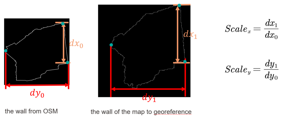
* '''Scaling''' | * '''Scaling''' | ||
[[File:Scaling.png| | The method to do scaling is shown in the image below. | ||
[[File:Scaling new.png|900px|thumb|center|Figure 8: An approximate scaling]] | |||
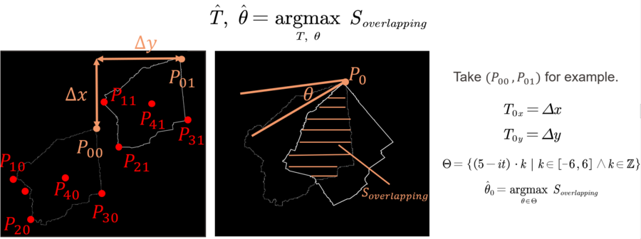
* '''Translation & Rotation''' | * '''Translation & Rotation''' | ||
[[File:Translation and | The goal of the translation and rotation is to obtain optimal translation and rotation to maximize the overlapping area of the two polygons. Since it’s computationally expensive to search for the translation pixel by pixel, and the angle degree by degree, we here narrow down the search space to translations that can fit the key point pairs respectively together (up-left points, up-right points, bottom-left points, bottom-right points and the centroids) and rotation angle set, which starts with [-30, 30] of step 5 and whose range and step will get smaller after every iteration (it's intuitive since after one iteration, we will need more accurate rotation angles). | ||
For every translation, we fix the key point together, rotate the wall and calculate the overlapping area. To calculate the overlapping area, we use the FloodFill algorithm to fill the area bounded by the source polygon and reference polygon respectively and use the logical-and operation to obtain the overlapping region. We then count the number of pixels that are not zero to be the overlapping area. | |||
After the iterations, we get the maximized overlapping area and the coordinates of the source polygon as well as the four vertices of the source image in the coordinate system of the reference image. | |||
[[File:Translation and Rotation new.png|900px|thumb|center|Figure 9: Translation and rotation]] | |||
===Coordinate System Transformation=== | |||
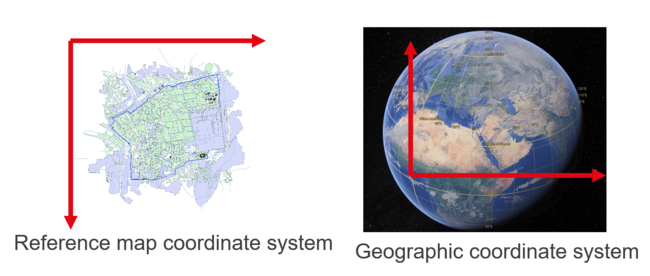
Since the final goal is to get the latitudes and longitudes in the geographic coordinate system of the four vertices of the raw maps, we finally transformed the coordinates of the image patches in the reference image coordinate system to the latitudes and longitudes of the raw maps through mathematical computations. | |||
[[File:Coordinate system transformation.png|650px|thumb|center|Figure 10: Coordinate System Transformation]] | |||
==Results== | ==Results== | ||
===Wall Extraction=== | ===Wall Extraction=== | ||
For the wall extraction step, the neural network gives good predictions. | For the wall extraction step, the neural network generally gives good predictions. | ||
{|class="wikitable" style="margin: 1em auto 1em auto;" | {|class="wikitable" style="margin: 1em auto 1em auto;" | ||
|- | |- | ||
| [[File: | | [[File:1837 contour.jpg|250px|thumb|center|Figure 11: Predicted contour of 1837]] | ||
| [[File: | | [[File:1845 contour.jpg|250px|thumb|center|Figure 12: Predicted contour of 1845]] | ||
| [[File:1883 contour.jpg|250px|thumb|center|Figure 13: Predicted contour of 1883]] | |||
| [[File:1921 contour.jpg|250px|thumb|center|Figure 14: Predicted contour of 1921]] | |||
|} | |||
But for some maps, there are some concavity and convexity in the predictions, but these flaws won't influence the alignment as shown in the next section. | |||
{|class="wikitable" style="margin: 1em auto 1em auto;" | |||
|- | |- | ||
| [[File: | | [[File:1853 3 contour.jpg|250px|thumb|center|Figure 15: Predicted contour of 1853]] | ||
| [[File: | | [[File:1855 contour.jpg|250px|thumb|center|Figure 16: Predicted contour of 1855]] | ||
| [[File:1920 contour.jpg|250px|thumb|center|Figure 17: Predicted contour of 1920]] | |||
| [[File:1929 contour.jpg|250px|thumb|center|Figure 18: Predicted contour of 1929]] | |||
|} | |||
===Wall Alignment=== | |||
For good predictions in the previous segmentation step, the alignment algorithm can give a satisfying alignment. | |||
{|class="wikitable" style="margin: 1em auto 1em auto;" | |||
|- | |||
| [[File:1883 contour.jpg|250px|thumb|center|Figure 19: Predicted contour of 1883]] | |||
| [[File:1921 contour.jpg|250px|thumb|center|Figure 20: Predicted contour of 1921]] | |||
|- | |||
| [[File:1883 predict.jpg|250px|thumb|center|Figure 21: Predicted contour of 1883]] | |||
| [[File:1921 predict.jpg|250px|thumb|center|Figure 22: Predicted contour of 1921]] | |||
|} | |||
The bias generally is caused by the intrinsic difference of the wall in the original map and the reference wall. The maps whose wall polygons have large differences from the nowadays wall polygon were generally produced in the early 19 century. Take the map in 1837 and 1845 for example. | |||
{|class="wikitable" style="margin: 1em auto 1em auto;" | |||
|- | |- | ||
| [[File: | | [[File:1837 contour.jpg|250px|thumb|center|Figure 23: Predicted contour of 1837]] | ||
| [[File: | | [[File:1845 contour.jpg|250px|thumb|center|Figure 24: Predicted contour of 1845]] | ||
|- | |||
| [[File:1837 predict.jpg|250px|thumb|center|Figure 25: Alignment result of 1837]] | |||
| [[File:1845 predict.jpg|250px|thumb|center|Figure 26: Alignment result of 1845]] | |||
|} | |||
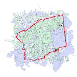
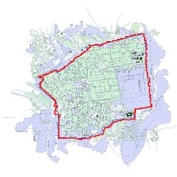
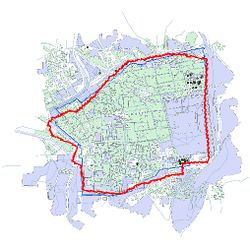
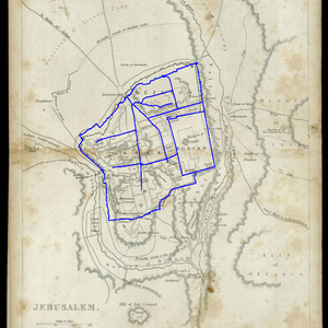
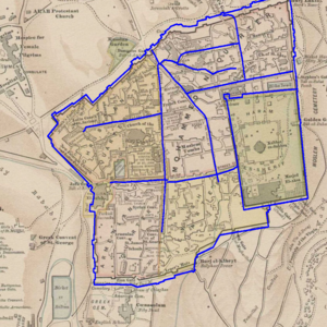
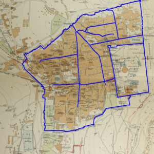
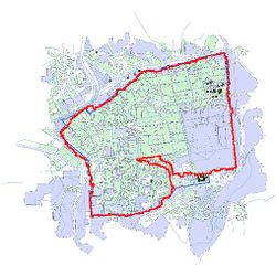
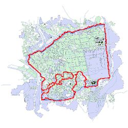
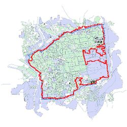
We add the main road from OpenStreetMap to the reference map and align them to the historical maps. The result also shows that the alignment results of more recent maps are better. | |||
{|class="wikitable" style="margin: 1em auto 1em auto;" | |||
|- | |- | ||
| [[File: | |[[File:1845 2cropped.png|300px|thumb|center|Figure 27: Alignment result of 1845]] | ||
| [[File: | |[[File:1887.png|300px|thumb|center|Figure 28: Alignment result of 1887]] | ||
|[[File:1915.png|300px|thumb|center|Figure 29: Alignment result of 1915]] | |||
|} | |} | ||
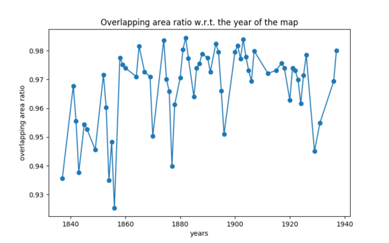
We | We plotted the overlapping area ratio with regard to the year of the map and find that the alignment result of early 19 century's maps are not as good as that of later maps, which is consistent with our previous observations. | ||
[[File:Curve.png|550px|thumb|center|Figure 30: Overlapping area ratio w.r.t the year of map]] | |||
Even for some maps with not that satisfying prediction results, the robustness of the alignment algorithms proposed make the polygons generally align together, thus the coordinates obtained are still reliable. | |||
{|class="wikitable" style="margin: 1em auto 1em auto;" | {|class="wikitable" style="margin: 1em auto 1em auto;" | ||
|- | |- | ||
|[[File: | | [[File:1853 3 contour.jpg|250px|thumb|center|Figure 31: 1853 contour]] | ||
|[[File: | | [[File:1855 contour.jpg|250px|thumb|center|Figure 32: 1855 contour]] | ||
|[[File: | | [[File:1920 contour.jpg|250px|thumb|center|Figure 33: 1920 contour]] | ||
| [[File:1929 contour.jpg|250px|thumb|center|Figure 34: 1929 contour]] | |||
|- | |||
| [[File:1853 3 predict.jpg|250px|thumb|center|Figure 35: 1853 predict]] | |||
| [[File:1855 predict.jpg|250px|thumb|center|Figure 36: 1855 predict]] | |||
| [[File:1920 predict.jpg|250px|thumb|center|Figure 37: 1920 predict]] | |||
| [[File:1929 predict.jpg|250px|thumb|center|Figure 38: 1929 predict]] | |||
|} | |} | ||
===Coordinate System Transformation=== | |||
The results are stored in a csv file shown as follows. | |||
[[File:Coordinate transformation.png|900px|thumb|center|Figure 39: Coordinates of the vertices of the raw map in geographic coordinate system]] | |||
==Limitations== | |||
- Although the alignment algorithm is not sensitive to the minor flaws of the segmentation results, the alignment performance is still subject to the segmentation results. Specifically, when the segmentation gives very bad predictions, the alignment algorithm just can't work. | |||
- The project can only do linear transformation, i.e. scaling, translation and rotation, but it can't do deformation. | |||
- Only the closed polygon of the wall are utilized and segmented. The morphological feature of road networks and buildings can also be exploited in future works. | |||
==Project Plan and Milestones== | ==Project Plan and Milestones== | ||
===Milestones=== | ===Milestones=== | ||
* Do survey on semantic segmentation and registration algorithms, get familiar with our dataset and decide what feature to be used for alignment. | *Do survey on semantic segmentation and registration algorithms, get familiar with our dataset and decide what feature to be used for alignment. | ||
* Preprocess the dataset. | |||
* Annotate the maps and use dhSegment for segmentation. | *Preprocess the dataset. | ||
* Design and implement the alignment algorithms. | |||
* | *Annotate the maps and use dhSegment for segmentation. | ||
*Design and implement the alignment algorithms. | |||
*Do coordinate system transformation. | |||
*Further improve the robustness of the alignment algorithm and connect the processing steps. | |||
*Sort out the code and write the report. | |||
===Plans=== | ===Plans=== | ||
| Line 138: | Line 268: | ||
| | | | ||
* Produce more wall-annotated images. | * Produce more wall-annotated images. | ||
* Fine-tune the dhSegment model to get better | * Fine-tune the dhSegment model to get better segmentation results. | ||
| align="center" | | | align="center" | ✓ | ||
|- | |- | ||
|By Week 12 | |By Week 12 | ||
| | | | ||
* Further improve the performance and robustness of the alignment algorithm to make it robust to poorly predicted data. | * Further improve the performance and robustness of the alignment algorithm to make it robust to poorly predicted data. | ||
* Transform the coordinates of the image patches in the reference image coordinate system to the latitudes and longitudes of the raw maps. | |||
* Make all the processing steps a pipeline and user-friendly. | * Make all the processing steps a pipeline and user-friendly. | ||
| align="center" | | | align="center" | ✓ | ||
|- | |- | ||
|By Week 13 | |By Week 13 | ||
| | | | ||
* Sort out the codes and push them to GitHub repository. | * Sort out the codes and push them to GitHub repository. | ||
* Write project report. | * Write the project report. | ||
* Prepare slides for final presentation. | * Prepare slides for final presentation. | ||
| align="center" | | | align="center" | ✓ | ||
|- | |- | ||
|By Week 14 | |By Week 14 | ||
| Line 161: | Line 292: | ||
|- | |- | ||
|} | |} | ||
==Github Link== | ==Github Link== | ||
https://github.com/mzp0514/JerusalemGeoreferencing | |||
==References== | ==References== | ||
[1] Oliveira, Sofia Ares, Benoit Seguin, and Frederic Kaplan. "dhSegment: A generic deep-learning approach for document segmentation." 2018 16th International Conference on Frontiers in Handwriting Recognition (ICFHR). IEEE, 2018. | |||
Latest revision as of 21:42, 20 December 2021
Motivation
The creation of large digital databases on urban development is a strategic challenge, which could lead to new discoveries in urban planning, environmental sciences, sociology, economics, and in a considerable number of scientific and social fields. Digital geohistorical data can also be used and valued by cultural institutions. These historical data could also be studied to better understand and optimize the construction of new infrastructures in cities nowadays, and provide humanities scientists with accurate variables that are essential to simulate and analyze urban ecosystems. Now there are many geographic information system platforms that can be directly applied, such as QGIS, ARCGIS, etc. How to digitize and standardize geo-historical data has become the focus of research. We hope to propose a model that can associate geographic historical data with today's digital maps, analyze and study them under the same geographic information platform, same coordinate projection, and the same scale. Eventually, it can eliminate errors caused by scaling, rotation, and the deformation of the map carrier that may exist in historical data and the entire process is automated and efficient.
The scale is restricted to Jerusalem in our project. Jerusalem is one of the oldest cities in the world and is considered holy to the three major Abrahamic religions—Judaism, Christianity, and Islam. We did georeferencing among Jerusalem’s historical maps from 1840 to 1949 and the modern map from OpenStreetMap so that the overlaid maps will reveal changes over time and enable map analysis and discovery. We focused on the wall of the Old City as the morphological feature to do georeferencing because the region outside the Old City has seen many new constructions while the Old City has not great changes and the closed polygon of the wall is relatively more consistent than other features like road networks. More specifically, we used dhSegment, a historical document segmentation tool, to extract the wall of the Old City of Jerusalem and proposed an alignment algorithm exploiting the geometrical features of the wall to align the maps.
Deliverables
- The latitudes and longitudes of the four vertices of the raw maps.
- Preprocessed (cropped and resized) patches of the raw maps with images information (including the position of the sub-image in the raw map) stored in a csv file.
- 42 1000 * 1000 annotations of the Old City area.
- Trained segmentation model.
- Code and instructions to reproduce the results on github.
Methodology
Dataset
- 126 historical maps of Jerusalem from 1837 to 1938.
- Modern geographical data of Jerusalem from OpenStreetMap.
Wall Extraction
We first used dhSegment to do image segmentation in order to extract the wall polygon from the maps. dhSegment [1] is a generic approach for Historical Document Processing, which relies on a Convolutional Neural Network to predict pixelwise characteristics. The whole process include preprocessing, training, predicting and postprocessing.
- Preprocessing
To make the image data fit into the neural networks and to make the old city region more dominant in the image, we cropped and scaled the original image by hand for subsequent uses.
- Map annotating
We used Procreate to pixel-wisely label 42 maps according to whether the pixel belong to the old city with different colors (RGB(0, 0, 0) for pixels inside the wall, RGB(255, 0, 255) for pixels outside the wall).
- Training
We divided the 42 annotated patches into 36 and 6 for training and validating respectively, and trained the model with learning rate 5e-5, batch size: 2, N_epochs: 40, and data augmentation like rotation, scaling and color.
- Prediction
By doing prediction on the testing set, we got the predicted old city region and naturally got the contour of it, i.e. the wall.
- Postprocessing
We removed the minor noises by retain the largest connected region and drew the contour of it. We put the contour on the original image and find that it generally fits well, although there are some minor deviations.
Wall Alignment
After obtaining the wall polygons, we try to fit them to the the reference wall polygon from the OpenStreetMap and obtain the coordinates of the source polygon as well as the four vertices of the source image in the coordinate system of the reference image.
- Overview
The overall algorithm proposed is shown as follows. We do scaling, transformation and rotation iteratively for a given iteration numbers in order to get a better alignment result since the initial scaling isn't the accurate enough with the angle difference of the source polygon and reference polygon.
- For i = 0 to iters :
- Estimate and do scaling
- For each point pair P in selected point pair set:
- Calculate and do transformation
- For k = -6 to 6 :
- Do rotation of angle = k(iters - i) around P
- Calculate overlapping area
- Update maximum overlapping area
- Scaling
The method to do scaling is shown in the image below.
- Translation & Rotation
The goal of the translation and rotation is to obtain optimal translation and rotation to maximize the overlapping area of the two polygons. Since it’s computationally expensive to search for the translation pixel by pixel, and the angle degree by degree, we here narrow down the search space to translations that can fit the key point pairs respectively together (up-left points, up-right points, bottom-left points, bottom-right points and the centroids) and rotation angle set, which starts with [-30, 30] of step 5 and whose range and step will get smaller after every iteration (it's intuitive since after one iteration, we will need more accurate rotation angles).
For every translation, we fix the key point together, rotate the wall and calculate the overlapping area. To calculate the overlapping area, we use the FloodFill algorithm to fill the area bounded by the source polygon and reference polygon respectively and use the logical-and operation to obtain the overlapping region. We then count the number of pixels that are not zero to be the overlapping area.
After the iterations, we get the maximized overlapping area and the coordinates of the source polygon as well as the four vertices of the source image in the coordinate system of the reference image.
Coordinate System Transformation
Since the final goal is to get the latitudes and longitudes in the geographic coordinate system of the four vertices of the raw maps, we finally transformed the coordinates of the image patches in the reference image coordinate system to the latitudes and longitudes of the raw maps through mathematical computations.
Results
Wall Extraction
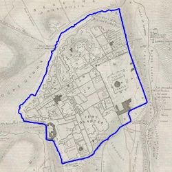
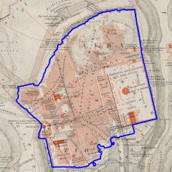
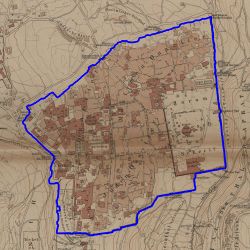
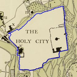
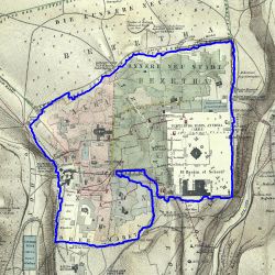
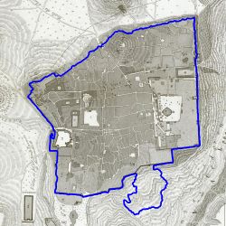
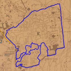
For the wall extraction step, the neural network generally gives good predictions.
But for some maps, there are some concavity and convexity in the predictions, but these flaws won't influence the alignment as shown in the next section.
Wall Alignment
For good predictions in the previous segmentation step, the alignment algorithm can give a satisfying alignment.
The bias generally is caused by the intrinsic difference of the wall in the original map and the reference wall. The maps whose wall polygons have large differences from the nowadays wall polygon were generally produced in the early 19 century. Take the map in 1837 and 1845 for example.
We add the main road from OpenStreetMap to the reference map and align them to the historical maps. The result also shows that the alignment results of more recent maps are better.
We plotted the overlapping area ratio with regard to the year of the map and find that the alignment result of early 19 century's maps are not as good as that of later maps, which is consistent with our previous observations.
Even for some maps with not that satisfying prediction results, the robustness of the alignment algorithms proposed make the polygons generally align together, thus the coordinates obtained are still reliable.
Coordinate System Transformation
The results are stored in a csv file shown as follows.
Limitations
- Although the alignment algorithm is not sensitive to the minor flaws of the segmentation results, the alignment performance is still subject to the segmentation results. Specifically, when the segmentation gives very bad predictions, the alignment algorithm just can't work.
- The project can only do linear transformation, i.e. scaling, translation and rotation, but it can't do deformation.
- Only the closed polygon of the wall are utilized and segmented. The morphological feature of road networks and buildings can also be exploited in future works.
Project Plan and Milestones
Milestones
- Do survey on semantic segmentation and registration algorithms, get familiar with our dataset and decide what feature to be used for alignment.
- Preprocess the dataset.
- Annotate the maps and use dhSegment for segmentation.
- Design and implement the alignment algorithms.
- Do coordinate system transformation.
- Further improve the robustness of the alignment algorithm and connect the processing steps.
- Sort out the code and write the report.
Plans
| Date | Task | Completion |
|---|---|---|
| By Week 4 |
|
✓ |
| By Week 6 |
|
✓ |
| By Week 8 |
|
✓ |
| By Week 10 |
|
✓ |
| By Week 11 |
|
✓ |
| By Week 12 |
|
✓ |
| By Week 13 |
|
✓ |
| By Week 14 |
|
-- |
Github Link
https://github.com/mzp0514/JerusalemGeoreferencing
References
[1] Oliveira, Sofia Ares, Benoit Seguin, and Frederic Kaplan. "dhSegment: A generic deep-learning approach for document segmentation." 2018 16th International Conference on Frontiers in Handwriting Recognition (ICFHR). IEEE, 2018.
