Reconstruction of Partial Facades: Difference between revisions
No edit summary |
Oscar.goudet (talk | contribs) |
||
| Line 104: | Line 104: | ||
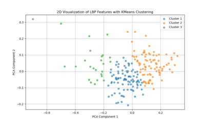
The two-dimensional projection of LBP features via PCA suggests that the textural characteristics of Venetian facades span a broad and continuous range, rather than forming a few discrete, well-defined clusters. Each point represents the LBP-derived texture pattern of a given image region or facade sample, and their spread across the plot indicates variation in texture complexity, detailing, and material transitions. If there were strong, distinct groupings in this PCA space, it would imply that certain facade types or architectural features share very similar texture signatures. Instead, the relatively diffuse distribution implies that Venetian facades exhibit a wide spectrum of subtle texture variations, with overlapping ranges of structural and decorative elements rather than neatly separable categories. | The two-dimensional projection of LBP features via PCA suggests that the textural characteristics of Venetian facades span a broad and continuous range, rather than forming a few discrete, well-defined clusters. Each point represents the LBP-derived texture pattern of a given image region or facade sample, and their spread across the plot indicates variation in texture complexity, detailing, and material transitions. If there were strong, distinct groupings in this PCA space, it would imply that certain facade types or architectural features share very similar texture signatures. Instead, the relatively diffuse distribution implies that Venetian facades exhibit a wide spectrum of subtle texture variations, with overlapping ranges of structural and decorative elements rather than neatly separable categories. | ||
Revision as of 15:42, 18 December 2024
Introduction
Motivation
The reconstruction of Venetian building facades is an interdisciplinary challenge, combining computer science, computer vision, the humanities, and architectural studies. Machine Learning (ML) and Deep Learning (DL) techniques offer a powerful solution to fill gaps in 2D facade data for historical preservation and visualization.
Facades vary significantly in structure, size, and completeness, making classical interpolation and rule-based methods inefficient. The Masked Autoencoder (MAE), a Transformer-based model, excels at learning patterns from large datasets and efficiently reconstructing missing regions. With its high masking ratio of 0.75, the MAE can learn robust representations while reconstructing large portions of missing data, making it seem ideal for processing the thousands of facades available to us in our dataset. The MAE captures both high-level structures (e.g., windows, arches) and fine details (e.g., textures, edges) by learning hierarchical features. Thus, it appears ideal for addressing the challenge of maintaining the architectural integrity of reconstructions, preserving stylistic elements crucial for historical analysis.
Venetian facades are valuable artifacts of cultural heritage. The MAE's ability to reconstruct deteriorated or incomplete structures supports digital preservation, enabling scholars and the public to analyze and visualize architectural history. By automating the reconstruction process, the MAE ensures scalable and accurate preservation of these historical assets. The Masked Autoencoder’s adaptability, scalability, and masking ratio of 0.75 make it uniquely suited to this reconstruction project. It efficiently handles large datasets, captures architectural details, and supports the digital preservation of Venice's rich cultural heritage.
Deliverables
link to the Github respository :
Project Timeline & Milestones
| Timeframe | Goals | Tasks |
|---|---|---|
| Week 4 |
|
|
| Week 5 |
|
|
| Week 6 |
|
|
| Week 7 |
|
|
| Week 8 |
|
|
| Week 9 |
|
|
| Week 10 |
|
|
| Week 11 |
|
|
| Week 12 |
|
|
| Week 13 |
|
|
| Week 14 |
|
|
Exploratory Data Analysis
To gain deeper insights into the architectural and typological properties of Venetian facades, we conducted a series of exploratory textural and color analyses, including Local Binary Patterns (LBP), Histogram of Oriented Gradients (HOG), Gabor filters, and color distribution examinations. These will provide supportive evidence for the choice of models, hyperparameters and error analysis.
Local Binary Pattern
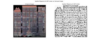
Local Binary Pattern (LBP) encodes how the intensity of each pixel relates to its neighbors, effectively capturing small-scale variations in brightness patterns across the surface. For the facade, this means LBP highlights areas where texture changes—such as the edges around windows, decorative elements, or shifts in building materials—are more pronounced. As a result, LBP maps reveal where the facade’s texture is smooth, where it becomes more intricate, and how these features repeat or vary across different sections of the building.
The two-dimensional projection of LBP features via PCA suggests that the textural characteristics of Venetian facades span a broad and continuous range, rather than forming a few discrete, well-defined clusters. Each point represents the LBP-derived texture pattern of a given image region or facade sample, and their spread across the plot indicates variation in texture complexity, detailing, and material transitions. If there were strong, distinct groupings in this PCA space, it would imply that certain facade types or architectural features share very similar texture signatures. Instead, the relatively diffuse distribution implies that Venetian facades exhibit a wide spectrum of subtle texture variations, with overlapping ranges of structural and decorative elements rather than neatly separable categories.
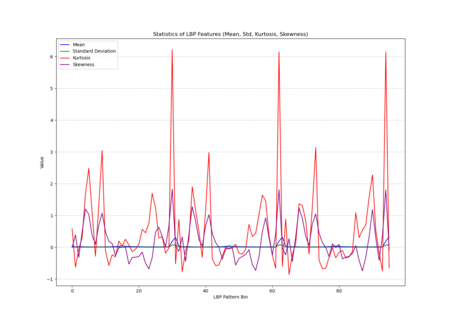
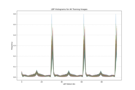
The histogram plot, displaying LBP distributions for all training images, shows pronounced peaks at certain pattern bins rather than a uniform or random spread, indicating that specific local texture patterns are consistently prevalent across the facades. The statistical plot (mean, standard deviation, kurtosis, skewness) further reveals that these patterns are not normally distributed; some bins have notably high kurtosis and skewness, indicating that certain textures appear more frequently and in a more clustered manner than others. In other words, Venetian facades are characterized by stable, repetitive textural signatures—likely reflecting repeated architectural elements and material arrangements—rather than exhibiting uniformly varied surface textures.
Gabor Filter
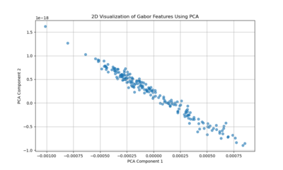
Gabor filters capture localized frequency and orientation components of an image’s texture. The PCA projection resulting in a near-linear distribution of points suggests that variation in the Gabor feature space is largely dominated by a single principal direction or a narrow set of related factors. This could imply that Venetian facades have a relatively uniform textural pattern, strongly influenced by a consistent orientation or repetitive decorative elements. In other words, the facades’ texture patterns may be comparatively regular and structured, leading to a low-dimensional representation where one main factor (like a dominant orientation or repetitive structural motif) explains most of the variation.
histogram of oriented gradients (HOG)
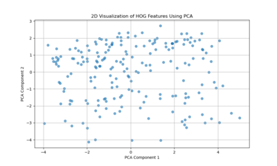
Histogram of Oriented Gradients (HOG) features capture edge directions and the distribution of local gradients. The more scattered PCA plot indicates that no single dimension dominates the variability as strongly as in the Gabor case. Instead, Venetian facades exhibit a richer diversity of edge and shape information — windows, balconies, ornaments, and varying architectural details produce a more heterogeneous distribution of gradient patterns. This complexity results in a PCA space without a clear linear trend, reflecting more complexity and variety in structural features and contour arrangements.
In Summary:
Gabor Features: Suggest a more uniform, repetitive texture characteristic of Venetian facades, possibly reflecting dominant architectural rhythms or orientation patterns.
HOG Features: Highlight a more diverse set of edge and shape variations, indicating that while texture may be consistent, the facades have numerous structural details and differing configurations that result in a more dispersed feature representation.
Together, these indicate that Venetian facades are simultaneously texturally coherent yet architecturally varied in their structural details.
I have this code in my wiki but the images are overalping in the next section , how to make sure this doesnt happen
Methodology
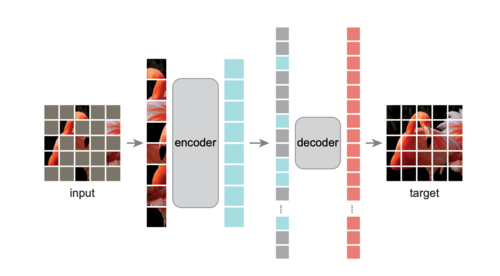
This project is inspired by the paper "Masked Autoencoders Are Scalable Vision Learners" by He et al., from Facebook AI Research (FAIR). The Masked Autoencoder splits an image into non-overlapping patches and masks a significant portion (40% to 80%) of them. The remaining visible patches are passed through an encoder, which generates latent representations. A lightweight decoder then reconstructs the entire image, including the masked regions, using these latent features and position embeddings of the masked patches.
The model is trained using a reconstruction loss (e.g., Mean Squared Error) computed only on the masked patches. This ensures the model learns to recover unseen content by leveraging contextual information from the visible patches. The simplicity and efficiency of this approach make MAE highly scalable and effective for pretraining Vision Transformers (ViTs) on large datasets.
By masking a substantial part of the image, MAEs force the model to capture both global structure and local details, enabling it to learn rich, generalizable visual representations.
For this project, two types of MAEs were implemented:
1) Custom MAE: Trained from scratch, allowing flexibility in input size, masking strategies, and hyperparameters.
2) Pretrained MAE: Leveraged a pretrained MAE, which was finetuned for our specific task.
Custom MAE
Data Preprocessing
Images were resized to a fixed resolution (e.g., 224x224) and normalized to have pixel values in the range [-1, 1] and the input image was divided into patches of size 8x8, resulting in a grid of 32x32 patches for each image.
Model Architecture
Encoder: The encoder takes visible (unmasked) patches as input and processes them using a Vision Transformer (ViT)-based architecture. Positional embeddings are added to the patch embeddings to retain spatial information. The encoder produces a latent representation for the visible patches.
Decoder: The decoder takes both the encoded representations of visible patches and learnable masked tokens as input. It reconstructs the image by predicting pixel-level details for the masked patches.
Masking Strategy
A contiguous block of patches is masked to simulate occlusion, which more accurately represents the incomplete facades in our data compared to a random masking strategy. A masking ratio of 50% was applied, meaning half of the patches in each image were masked during training.
Loss Function
To optimize the model, I used a combination of Masked MSE Loss and Perceptual Loss. The Masked MSE Loss, following the original MAE methodology, is computed only on the masked patches to encourage reconstruction of unseen regions. The Perceptual Loss, derived from a pre-trained VGG19 network, enhances reconstruction quality by focusing on perceptual similarity, also restricted to masked regions. The final loss is a weighted combination:
\mathcal{L} = 0.6 \cdot \text{MSE Loss} + 0.4 \cdot \text{Perceptual Loss}
Training and Optimization
The model was trained using the AdamW optimizer, with a learning rate scaled based on batch size and a cosine decay scheduler for gradual reduction of learning rates. A warm-up phase was incorporated to stabilize training during the initial epochs.
Evaluation Metrics
Performance was evaluated based on reconstruction quality (MSE + perceptual loss) and visual fidelity of reconstructed images.
Pre-Trained MAE
NMF
The incentive to use Nonnegative Matrix Factorization (NMF) for facade image reconstruction is based on several key points: 1) NMF provides a relatively simple and easily adjustable model structure; 2) NMF can handle outliers and noises more effectively than certain complex models. 3) The loss function can be fully customized, allowing future incorporation of semantic or textural-level loss, rather than relying purely on pixel-wise errors; 4) Compared to methods like Masked Autoencoders (MAE), NMF has significantly fewer hyperparameters, making the model more interpretable. This is particularly advantageous in contexts requiring cultural heritage preservation, where interpretability is paramount.
NMF factorizes a data matrix V into two lower-dimensional nonnegative matrices W and H such that: V &\approx W H, where W \in \mathbb{R}^{n \times k} and H \in \mathbb{R}^{k \times m}. The parameter k denotes the number of components (or latent features), chosen based on the desired level of detail. Each row of H corresponds to a learned component or “basis image,” and each row of W provides the coefficients that combine these components to approximate a given training image.
The factorization is typically achieved by minimizing an objective function (e.g., the Frobenius norm of the reconstruction error). By constraining both W and H to be nonnegative, NMF encourages parts-based representations. Each component tends to capture localized structural patterns—such as windows, edges, or balconies—that are commonly found in facades.
To reconstruct a new test image with missing regions, the same preprocessing steps (resizing, normalization, flattening) are applied. Missing pixels can initially be imputed with zero or another neutral value. The fitted NMF model is then used to project this incomplete test image onto the learned latent space: H_{\text{test}} = \text{nmf_model.transform}(V_{\text{test}}), where V_{\text{test}} is the vectorized incomplete image. The resulting H_{\text{test}} encodes the combination of learned components that best approximate the partially observed image.
The reconstructed image is obtained by: V_{\text{test reconstructed}} = H_{\text{test}} \times H.
Here, H represents the learned dictionary of facade patterns. Multiplying H_{\text{test}} by H reconstructs an image that fills in missing areas with patterns consistent with the training set. Finally, this reconstruction is reshaped into the original image dimensions.
While NMF-based reconstruction may not guarantee perfect results—especially if large portions of the image are missing or if the training set is not sufficiently diverse—it often yields more semantically meaningful completions than simple pixel-level interpolation. Potential improvements include integrating additional techniques (e.g., texture synthesis, advanced regularization) or incorporating prior architectural knowledge.
Hyperparameter Choice of NMF
1. Dimensionality Reduction Insights: • PCA Pre-analysis: Before running NMF, apply Principal Component Analysis (PCA) to the training and test images. Analyze the explained variance of PCA components to estimate the intrinsic dimensionality of the data. • Reconstruction Saturation: Determine a range of PCA components at which reconstruction quality stops improving significantly. This provides a strong initial guess for the number of components (n_components) in NMF. 2. Hyperparameter Decisions for NMF: • Number of Components (n_components): Choose a value informed by PCA and by evaluating the reconstruction performance. Strive to capture most of the variance without overfitting. (See figure of PCA explained variance) • Initialization (init): Use nndsvda (Nonnegative Double Singular Value Decomposition with zeroing) for faster convergence and better initial component estimates. • Regularization: Consider adding L1 or L2 regularization (via l1_ratio) to promote sparsity or smoothness in the learned components. Decisions on regularization parameters can be guided by cross-validation or domain-specific considerations (e.g., promoting certain architectural features while discouraging noise).
Results
custom MAE
The results obtained from training our custom MAE were not entirely satisfactory, as the reconstructed images appeared quite blurry and lacked fine-grained details, having difficulty recovering features like windows or edges. The original motivation for training the model from scratch was to have greater flexibility in the model architecture. By building a custom MAE, we aimed to tailor the model's design to the specific challenges of our dataset, such as the unique structure of incomplete facades and the need to experiment with different parameters like masking strategies, patch sizes, and embedding dimensions. This level of customization allowed us to explore architectural decisions that might better align with the characteristics of our data, compared to relying on a pretrained model with fixed design choices but a major limitation in this setup was the size of the dataset, which contained only 650 images of complete facades. Training a deep learning model like an MAE, especially from scratch, requires a much larger dataset to effectively learn meaningful representations. With such a small dataset, the model struggled to generalize, focusing on coarse, low-frequency features such as the overall structure and color distribution, rather than capturing finer details like edges, textures, and patterns.
While perceptual loss based on VGG19 features did improve the reconstruction quality, its impact remained constrained by the small size of the training set. The model began to recover higher-level patterns and global structures, but lacked the fine-grained detail that would be possible with more extensive training data.
To overcome these limitations, we opted to use a pretrained model instead of training from scratch. The pretrained model, fine-tuned on our specific dataset, leveraged learned representations from large-scale training on diverse data, allowing it to generalize much better. By building on the rich, low- and high-level features already embedded in the pretrained network, the fine-tuned model produced significantly sharper and more realistic reconstructions. In the next section, we will present the results obtained using this pretrained model, highlighting its improved performance compared to the custom MAE.
Error Analysis
Linking Feature Representations to MAE Reconstruction
Gabor Features:
These features highlight repetitive, uniform texture patterns. Venetian facades often have recurring motifs—brick patterns, stone arrangements, or consistent color gradients. The Gabor analysis showed that the facades, in terms of texture frequency and orientation, vary along a mostly one-dimensional axis, suggesting a strong commonality.
Implication for MAE:
Since MAEs learn to fill in missing patches by leveraging global context, regular and repetitive textures are easier to guess. If part of a patterned surface (like a uniform wall area) is masked, the MAE can infer what belongs there from the context it has learned. As a result, reconstruction errors on these uniform, texturally consistent regions are likely to be low.
HOG Features:
HOG captures edge distributions, corners, and the shapes formed by architectural details—think windows, balconies, ornate moldings, and decorative columns. The PCA results for HOG were more scattered, indicating that Venetian facades do not have a single dominant “type” of edge pattern, but rather a wide variety of distinct and intricate details.
Implication for MAE:
Irregular, unique details are harder for the MAE to predict if they’re masked. Unlike repetitive textures, a unique balcony shape or an uncommon decorative element can’t be inferred as easily from nearby patches. The MAE may reconstruct something plausible in broad strokes but miss subtle intricacies, leading to higher error in these regions.
1. Structural Regularity and Symmetry
LBP analysis reveals pervasive repeating patterns and structural symmetry, providing a reference for understanding Masked Autoencoder (MAE) reconstructions. The MAE excels at reproducing these large-scale patterns—such as window alignments or arch sequences—aligning closely with LBP findings that emphasize overarching geometric coherence.
2. Texture Simplification
LBP indicates where surfaces transition from smooth to intricate textures. While these findings highlight the presence of finely detailed regions, the MAE reconstructions tend to simplify such areas. The loss of subtle textures arises from the MAE’s focus on recovering global structure rather than capturing every local nuance—an inherent limitation that LBP helps explain.
3. Smooth vs. High-Detail Areas
LBP distinctions between smooth and heavily ornamented areas correspond directly to MAE outcomes. Smooth surfaces, easily modeled due to their low variance, are faithfully reconstructed. In contrast, complex textures appear blurred, reflecting the MAE’s challenge in fully restoring the fine-scale intricacies that LBP so clearly delineates.
4. Hierarchical Architectural Features
LBP’s highlight of hierarchical architectural arrangements explains how the MAE manages certain architectural features well (e.g., aligning windows and maintaining facade outlines) while struggling with finer ornamental elements. This hierarchical perspective helps us understand why global forms are preserved, whereas delicate details fade.
Future Direction
Conclusion
Appendix
References
He, K., Chen, X., Xie, S., Li, Y., Dollár, P., & Girshick, R. (2022). Masked Autoencoders Are Scalable Vision Learners. Proceedings of the IEEE/CVF Conference on Computer Vision and Pattern Recognition (CVPR), 16000–16009. https://openaccess.thecvf.com/content/CVPR2022/papers/He_Masked_Autoencoders_Are_Scalable_Vision_Learners_CVPR_2022_paper.pdf
