Extracting Toponyms from Maps of Jerusalem

Introduction

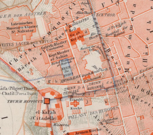
We aim to programmatically and accurately extract toponyms (place names) from historical maps of Jerusalem. Building from mapKurator, a scene text recognition pipeline developed specifically for toponym extraction by the University of Minnesota's Knowledge Computing Lab, we develop a novel label extraction and processing pipeline capable of significant accuracy improvements relative to mapKurator's spotter module alone. We then explore the success of our pipeline during generalization, describe the limitations of our approach, and suggest possibilities for future progress in accuracy or end-user interactivity.

Motivation

A sample of the linguistic, geometrical, and typographical diversity of toponyms in 19th-century maps of Jerusalem.

Development of an accurate, accessible, and generally applicable tool for extraction of map toponyms is an unrealized goal. Indeed, despite the deep-learning induced boon to scene text recognition (STR) seen in the past decade, STR in general remains difficult due to the sheer variety of shapes, fonts, colors, languages, and text backgrounds encountered. In the context of historical maps and Jerusalem especially, STR issues are compounded by the fact that there is not necessarily agreement between cartographers over toponym spellings (in the case of toponyms transliterated from arabic, for example) or, as is true among biblical toponyms, even the precise location of certain places. Properly collecting toponym locations and spellings from historical maps of Old Jerusalem would thus permit researchers to understand how such ambiguities have manifested as agreement or disagreement in geographic depiction throughout time.

In an effort to automate text recognition on historical map archives - our exact use case - the University of Minnesota's Knowledge Computing Lab has developed an end-to-end toponym extraction and rectification pipeline dubbed mapKurator. While we do build on their methods, we identify three issues with simply implementing mapKurator on historical maps of Jerusalem to achieve our intended result. First, some elements of the full mapKurator pipeline (namely the use of Open Street Map to correct extracted labels) are not suitable for historical maps of Jerusalem due to the ambiguities described above. Second, the success of the chief tool used to extract text in mapKurator depends heavily on its model weights - weights that users may not have the computational power or ground truth labels to train. Third, mapKurator's text spotting tool only extracts individual words, requiring further processing to capture multi-word toponyms. We therefore decide to augment mapKurator's text spotting tool with a pipeline involving repeated sampling and methods for recovering proper toponyms from said sampling.

The contributions of this project are thus inroads into the collection of accurate toponyms from historical maps of Jerusalem and a general, accessible pipeline that can be mounted on a pre-trained STR label extractor to improve accuracy.

Deliverables

• A novel, general-use, and computationally accessible toponym extraction pipeline capable of improving accuracy for pre-trained SOTA neural network models.

• A set of X ground truth toponyms across 3 historical maps of Jerusalem.

• A set of X extracted toponyms across 3 historical maps of Jerusalem.

• A set of X labels denoting font similarity across 3 images of toponyms.

These deliverables are available via the Git repository linked at the bottom of this page.

Methodology

MapKurator Spotter

A sample of results from spotter-v2 network on a map of Jerusalem.

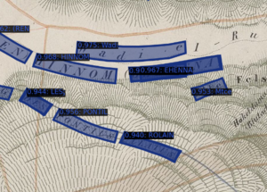
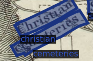
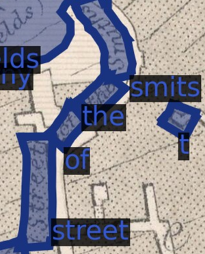
MapKurator's Spotter module is a neural network based methods of extracting text instances on scaned historical maps. Text instances are defined as a tuple of Bounding Polygon, Text and Confidence Score. The original mapKurator team proposed two networks, TESTR and spotter-v2, in our case, we decide to use spotter-v2 model.

Pyramid Scan

Cutting the original maps into small patches and feed the patches to the model is a economic and effective way of getting text instances from a large map. Original mapKurator team used a image crop step in their pipeline, however, this method is rather naive and crude. Cut with fixed pixel resolution make the pipeline suffer from the inability of adapting to different resolutions of scanned maps. This results in omitting text instances that the model could have spotted.

We proposed a pyramid structured images patches cut from the original map to address the aforementioned issue. The original images are cut into n by n image patches with 30% overlapping. We gradually increase n as we deepens the layers. Our experiments suggest 5 layers of pyramid guarantees a stable increase in all evaluation metrics while keeps a reasonable computational cost.

Extracted Label Processing

Subword Deduplication

Let the set ES^SG refer to the set of extracted word labels that correspond to ground-truth subword SG in its entirety. The goal of Subword Deduplication is to retain the single most accurate extracted word W in a given ES^SG and exclude the rest - to filter ES^SG such that there remains just one extracted `representative' for SG, in other words. Let σ^* be the single extracted label remaining in ES^SG after subword deduplication has occurred.

We begin by performing unsupervised clustering of extracted labels' bounding boxes into appropriate sets. To do so, we vectorize each extracted bounding box P with its bottom left and top right cartesian coordinates and implement DBSCAN on the resulting set of four-dimensional vectors. Regarding hyperparameters, we set the maximum distance possible between neighbors intra-cluster to 50 and the number of intra-neighborhood observations defining a core observation to be 3. Outliers identified by DBSCAN are excluded from further processing under the assumption that actual text (as opposed to noise) would be extracted multiple times under our pyramid approach and thus be slotted into a cluster.

With our set of geometric clusters available (meaning we have ES^SG for all SG apparently captured during extraction), we proceed to filter each set down to its most appropriate representative by observing extracted text (T) and confidence scores (C). If T is unique for all extracted words in ES^SG, then σ^* earns the T from the label for which C is highest. If T is not unique for all extracted words in ES, we first deduplicate instances of T by choosing one confidence score from a given text's associated confidence scores via a RANSAC search, then proceed as specified above.

We end this stage with a single σ^* for each SG apparently recognized by our model; call this set σ^*.

Nested Word Flattening

Let Σ^WG represent for a given ground truth word WG the set of extracted and deduplicated word labels amounting to all relevant unique subwords identified by our model. Note that for a given ground-truth word, the set of subwords captured by our model may or may not cover all possible subwords that can be derived. The goal of Nested Word Flattening is to retain a single label from each Σ^WG: the label ψ^* = WG.

This process is performed iteratively. The first step in the sequence consists of computing pairwise geometric and textual intersection over minimum (IoM) values between all labels in Σ^WG. For example, suppose we are comparing σ₁ and σ₂. In this case, geometric IoM equals P₁ ∩ P₂ (the intersection of the associated bounding box polygons) divided by the area of the smaller polygon. Textual IoM, meanwhile, equals the number of non-unique shared characters in label texts T₁ and T₂ divided by the length of the longer string. Those pairs with geometric IoM value γ_geom > 0.75 and textual IoM value γ_text > 0.5 are considered to exhibit a subset-parent relationship. They are therefore `flattened,' or amalgamated, meaning (1) a new word label σ_α is added to Σ^WG with P_α = P₁ ∪ P₂ and T_α equal to the longer string from T₁ and T₂, and (2) both σ₁ and σ₂ are dropped from Σ^WG. When all possible amalgamations have been made based on the group of pairwise combinations satisfying our γ_geom and γ_text conditions, the sequence begins anew with updated Σ^WG, and ultimately terminates when Σ^WG ceases to yield further possible amalgamations.

Once both Subword Deduplication and Nested Word Flattening have occurred, the set of extracted words W has been condensed to the set Ψ composed of each unique word label ψ^* considered equivalent to some ground truth word in the ground truth set.

Sequence Recovery

The biggest issue with steps until now is that they are "word" level extraction. This chapter is about how to recover a sequence of words (i.e., a phrase) from geometric features and typographical features from word snippets extracted from previous steps.

Identified toponyms patterns are "Single Lines", "Multiple Lines" and "Curved Lines". We are focusing on single line sequence recovery.

Single Line

Multiple Lines

Curved Line

Font Similarity

The archetecture of our Font Descriminator.

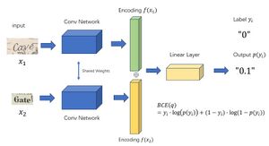
We assume that word labels which belong to a sequence are identical in their fonts. To implement this assumption, we train a neural network which takes as input two cropped images of text outputs a font similarity score between 0 and 1, i.e., the probability of two texts having the same font.

To train our model, we first crop rectangular images for all labels in G. By manually annotating randomly chosen image pairs and padding annotations with pairs that appear in multiline toponyms (assumed to have a similarity of 1), we create 447 matching-font labels and 2,022 non-matching-font labels. We used 80% of these labels to train our model, retaining the rest for testing. Our model achieved 92.9% recall and 89.7% precision on the test set.

As the image shows on the right shows, we implement a Siamese network which encodes two input images of text on a map (resized as 128*128) with the same two-layer convolution neural network, and use two linear layers and a Sigmoid function to map the concatenated vector of images to a scalar value ranging from 0 to 1. We use Binary Cross Entropy and the Adam optimizer with learning rate 0.01 for training, and retain the model weights obtained at epoch 40 for later use.

Once the model is trained, we calculate font similarity for all pairwise combinations of subword-deduplicated and nested-word-flattened word labels in Ψ.

Spline Connection Cost

Visualization of Bezier Splines on text instances.

Illustration of Bezier Splines.

Illustration of Spline Connection Cost.

We assume that word labels which belong to a sequence should be connectable via relatively short and non-curved splines. To implement this assumption, for each subword-deduplicated and nested-word-flattened word label ψ in Ψ, we first apply PCA to the points constituting bounding box P_ψ to recover unit vector d_ψ, the principal component basis for a given label's bounding box. Furthermore, for each P_ψ, we create the vectors e_ψ,p between successive points p in ℤ along P_ψ, recovering directional vectors along each label's bounding box. We then use these bounding-box vectors to adjust the principal component direction vector in preparation for spline calculation as follows:

Define RES_p = |d_ψ * e_ψ,p| (1 - |d_ψ * e_ψ,p|). For bounding-box vectors parallel or orthogonal to d_ψ, this value will be 0. Our goal is to maximize the number of vectors (nearly or exactly) parallel or orthogonal to d_ψ, as it would represent a more suitable principal direction for a given bounding box. Thus, our specific objective function is minimize the sum across all p of w_p*(RES_p)², where w_p is the length of e_ψ,p (it is more important for longer bounding box vectors to agree with the principal component direction than shorter bounding box vectors). We retrieve the optimal principal component direction d_ψ^* via the Gauss-Newton algorithm for solving non-linear least squares optimizations.

Next, for each d_ψ^*, we define a primary and secondary axis relative to the centroid of the associated bounding box P_ψ (the latter axis being orthogonal to d_ψ). We call this local axis the bounding box's anchor. If the variance of the principal component for a given bounding box is six times larger than the variance of the secondary component, we assume the polygon may have sufficient size to warrant different local axes at different locations (for example, the word may be curved), and thus, we divide the bounding box to permit multiple anchor points. These anchor points are points through which splines are drawn.

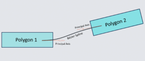
We create Cubic Bezier splines to measure the cost of connecting word labels. Assume we are drawing a spline from anchor point ξ₁ to anchor point ξ₂ in distinct word labels wl₁ and wl₂. The first control point cp₁ is the centroid of ξ₁. The second control point is cp₁ plus the product of (1) the furthest point from cp₁ on wl₁'s bounding box in ξ₁'s principal direction and (2) ξ₁'s principal direction vector. The fourth point cp₄ is of course the centroid of ξ₂, meaning the third control point is ξ₂ minus the product of (1) the furthest point from cp₄ on wl₂'s bounding box in ξ₂'s principal direction and (2) ξ₂'s principal direction vector. . We are, in effect, drawing a curve between two polygons that respects their orientation. After drawing such splines between all pairwise combinations of word labels (with distant geometric pairs excluded to reduce computational complexity), we can finally calculate the cost of connecting word labels via spline.

For a given spline, let C equal its maximum curvature, AD equal the euclidean distance between the two connected anchor points' centroids, and GD equal the minimum euclidean distance between two connected bounding boxes. The greater a spline's maximium curvature and the greater the distance between two polgyons, the less likely it is two polygons deserve to be grouped into a sequence. However, one should scale both quantities by centroid distance to achieve scale invariance. Hence, the Spline Connection cost is equal to C * AD * GD / AD = C * GD, which ranges from 0 to infinity. The smaller this value, the more it makes sense for two word labels to belong to the same sequence.

Combining Word Labels Using Font and Spline Metrics

With both font similarity and spline connection cost metrics in hand, we identify those word label pairs for which spline connection cost is less than 0.5 and for which font similarity is greater than 0.5. We then commence pairwise combinations by prioritizing the smallest spline connection costs; combined labels inherit maximum font similarity scores and minimum spline connection to constituent labels' neighbors, while text is concatenated starting with the leftmost polygon's text in a given pair. This process is performed iteratively until no combinations can be made, at which point the resultant set Θ is assumed to be equivalent to G (some issues with this assumption are discussed in the limitations section below).

Evaluation Metrics

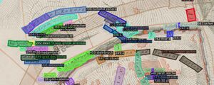
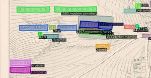
Unmentioned thus far is how we develop our ground truth label set G. Using the online image annotating software VIA, we manually label X labels across 3 maps. These 3 maps were chosen for their high resolution, their preponderance of toponyms located directly over place locations (as opposed to inside legends), their visual diversity, and their linguistic diversity. Ground truth labels are annotated at the line level rather than the toponym level. For example, if "Church of" appears directly above "the Flagellation", we annotate each as a separate ground truth label - though we manually indicate that they belong to the same toponym by assigning a group id. Line-level annotations with the option for multiline combination allows us to report accuracy statistics at both the line- and multiline-level, shedding light on the power of our pipeline in different contexts.

To evaluate Θ for a given map, we first retain only those extracted and processed labels located in the same pixel space as a crop of the map which has all possible ground truth toponyms in G. We then calculate all pairwise geometrical IoUs between these subsets of Θ and G, find the 1-to-1 matched set that maximizes the sum of said IoUs, and divide this sum by the number of extracted labels (in the case of precision) or the number of ground truth labels (in the case of recall). Text-based accuracy statistics, meanwhile, report the sum of normalized Levenshtein edit distances from the 1-to-1 geometrically matched set divided by the pertinent number of labels.

Results

A cropped image illustrating the final result for Kiepert 1845. Text instances from the same sequence have the same color.

A cropped image illustrating the final result for Saunders 1874. Text instances from the same sequence have the same color.

A cropped image illustrating the final result for Vandevelde 1846. Text instances from the same sequence have the same color.

Kiepert 1845 (111 ground truth labels)

	Precision		Recall
	Geometric	Textual	Geometric	Textual
Baseline	19.11%	8.62%	14.22%	6.42%
Pyramid + Processing	48.16%	47.71%	58.24%	57.69%

Saunders 1874 (136 ground truth labels)

	Precision		Recall
	Geometric	Textual	Geometric	Textual
Baseline	14.48%	13.59%	34.82%	32.68%
Pyramid + Processing	35.08%	31.57%	51.08%	45.97%

Vandevelde 1846 (94 ground truth labels)

	Precision		Recall
	Geometric	Textual	Geometric	Textual
Baseline	14.90%	9.60%	35.68%	22.95%
Pyramid + Processing	43.13%	44.71%	59.65%	61.84%

We see both precision and recall improvements at the text- and geometric-level across three distinct maps. Additionally, we find that, with but one exception, each stage of our processing pipeline provides a marginal boost to accuracy statistics across all three maps (these marginal statistics are not pictured). We are cautiously enthusiastic about our results, and use the next to section to discuss potential areas of weakness.

Limitations and Future Work

One chief limitation of our project is the limited evidence pointing toward its generalizability. With only 341 ground truth labels developed from 3 maps – maps chosen in part for their relatively high resolution – and marked inter-map variation in accuracy boosts, it is not evident that our pipeline would assuredly yield significant benefits across other historical maps of Jerusalem, not to mention other maps in general. Furthermore, defining our baseline as the accuracy of mapKurator’s pre-trained extraction module on historical maps of Jerusalem is problematic given that it was developed using a different map archive. A more appropriate evaluation regime would involve applying our pipeline to the same set of maps and labels the mapKurator team used to create and evaluate their model, thus expanding the number and diversity of ground truth labels, decoupling the marginal effect of our pipeline from the marginal effect of substituting the mapKurator’s map archive with another, and (ideally) making a stronger case for our pipeline’s generalizability. Though this evaluation regime is outside the scope of this Jerusalem-based project, we consider it to be the most important step toward the further validation of our approach.

Certain stages of our pipeline could benefit from further tuning. Our spline-based approach toward single line sequence recovery does not accommodate cases where the centroid of two consecutive words is vertically mismatched (such as when a small, short word follows a larger word and both are bottom-justified, for example). We neglect neglect multiline sequences in our current pipeline. One of our chosen maps uses a pervasive graphical element to represent trees that is consistently mistaken by the mapKurator spotter tool for a letter of text. Many such unresolved corner cases persist due to time limitations; addressing them would boost accuracy statistics. So too would developing further labels for font discriminator tool, which still misclassifies a small set of label pairs despite thousands of manually labelled comparisons, likely due to imbalance in the number of matching fonts in the label set. In fact, given the narrow map coverage and imbalanced label set used to train the discriminator, it may still take considerable signal from the map the text is pulled from rather than the type of font used alone. Identifying and tackling each processing stage’s distinct imperfections is a necessary if time-intensive path toward making our pipeline production ready.

Finally, we recognize that certain elements of the mapKurator pipeline which we disregard due to their inability to directly apply to our map archive would be beneficial if adapted for our project. We refer primarily to the PostOCR module, in which extracted text is mapped to verified toponyms from OpenStreetMap using a fuzzy query function (the issue with directly using this module is described in the Motivation section above). One can imagine emulating this process with a different set of “valid” toponyms: simply run the spotter module over a vast set of Jerusalem maps, apply our label processing pipeline, retain a set of the most prolific toponyms (or perhaps words) across all maps as the substitute for OpenStreetMap’s dictionary, and revisit all extracted toponyms to modify or at least annotate any which exhibit minor spelling changes from this novel dictionary. Such a process would invoke the same sampling justification behind the pyramid scanning regime to create a global, archive-wide dictionary in an unsupervised manner, create a lens through which to view potential spelling disagreements, and facilitate an environment in which our pipeline actually improves as more unlabeled data is processed.

We believe the pipeline we have produced to be useful and sound despite the limitations listed above, and are eager to see how resolving them might further improve the extraction of toponyms from historical maps.

Project Timeline

Timeframe	Task	Completion
Week 4	Finalize and present project proposals. Toponym extraction project selected.	✓
Week 5	Survey SOTA toponym extraction tools.	✓
Week 6	Port MapKurator's Spotter tool and model weights into Windows-based Python. Select two (later three) maps to use when implementing, evaluating, and fine-tuning MapKurator's model.	✓
Week 7	Create ground truth labels for first map with VIA's online interface.	✓
Week 8	Create ground truth labels for second map. Implement 1:1-matched precision and recall via IoU (geometry) and normalized Levenshtein (text). Calculate baseline accuracy statistics.	✓
Week 9	Implement multi-layer pyramid application of MapKurator's Spotter.	✓
Week 10	Create ground truth labels for third map. Implement subword deduplication and nested word flattening on pyramid-derived toponyms.	✓
Week 11	Calculate pyramid accuracy statistics. Fine-tune subword deduplication and nested word flattening. Deliver Midterm presentation.	✓
Week 12	Launch Wiki. Implement PCA on extracted label polygons to assist in font discriminator crops and Bezier splines. Create manual labels for font discriminator. Train font discriminator.	✓
Week 13	Add ground truth labels to our three maps. Implement Bezier spline Implement iterative sequence recovery using font and Bezier scores	✓
Week 14	Fine-tune Sequence Recovery. Calculate final accuracy statistics. Finalize Wiki and final presentation. Postponed for future work: Hierarchize final toponyms and develop Voronoi map. Prototype toponym-disagreement visualizer.	✓

Github Repository

Jerusalem Maps EPFL DH405

Acknowledgements

We thank Professor Frédéric Kaplan, Sven Najem-Meyer, and Beatrice Vaienti of the DHLAB for their valuable guidance over the course of this project.

References

Webpages

• MapKurator GitRepo
• MapKurator Introduction
• VIA Image Annotator

Chief Literature

• Kim, Jina, et al. "The mapKurator System: A Complete Pipeline for Extracting and Linking Text from Historical Maps." arXiv preprint arXiv:2306.17059 (2023).
• Li, Zekun, et al. "An automatic approach for generating rich, linked geo-metadata from historical map images." Proceedings of the 26th ACM SIGKDD International Conference on Knowledge Discovery & Data Mining. 2020