Venice2020 Building Heights Detection: Difference between revisions
| Line 441: | Line 441: | ||
| style="font-family:Arial, Helvetica, sans-serif !important;;" | 24.33m | | style="font-family:Arial, Helvetica, sans-serif !important;;" | 24.33m | ||
| style="font-family:Arial, Helvetica, sans-serif !important;;" | 23.21m | | style="font-family:Arial, Helvetica, sans-serif !important;;" | 23.21m | ||
| | | 4.82 | ||
| 11 | | 11 | ||
| 22m | | 22m | ||
| 23.21m | | 23.21m | ||
| | | 5.21 | ||
|- | |- | ||
| style="font-family:Arial, Helvetica, sans-serif !important;;" | 5 | | style="font-family:Arial, Helvetica, sans-serif !important;;" | 5 | ||
| style="font-family:Arial, Helvetica, sans-serif !important;;" | 26m | | style="font-family:Arial, Helvetica, sans-serif !important;;" | 26m | ||
| style="font-family:Arial, Helvetica, sans-serif !important;;" | 26.35m | | style="font-family:Arial, Helvetica, sans-serif !important;;" | 26.35m | ||
| | | 1.32 | ||
| 12 | | 12 | ||
| 11m | | 11m | ||
| 12.07m | | 12.07m | ||
| | | 8.86 | ||
|- | |- | ||
| style="font-family:Arial, Helvetica, sans-serif !important;;" | 6 | | style="font-family:Arial, Helvetica, sans-serif !important;;" | 6 | ||
| style="font-family:Arial, Helvetica, sans-serif !important;;" | 21m | | style="font-family:Arial, Helvetica, sans-serif !important;;" | 21m | ||
| style="font-family:Arial, Helvetica, sans-serif !important;;" | 22.21m | | style="font-family:Arial, Helvetica, sans-serif !important;;" | 22.21m | ||
| | | 5.44 | ||
| 13 | | 13 | ||
| 14m | | 14m | ||
| 14.18m | | 14.18m | ||
| | | 1.26 | ||
|- | |- | ||
| style="font-family:Arial, Helvetica, sans-serif !important;;" | 7 | | style="font-family:Arial, Helvetica, sans-serif !important;;" | 7 | ||
| style="font-family:Arial, Helvetica, sans-serif !important;;" | 21m | | style="font-family:Arial, Helvetica, sans-serif !important;;" | 21m | ||
| style="font-family:Arial, Helvetica, sans-serif !important;;" | 21.53m | | style="font-family:Arial, Helvetica, sans-serif !important;;" | 21.53m | ||
| | | 2.46 | ||
| 14 | | 14 | ||
| 16m | | 16m | ||
| 16.98m | | 16.98m | ||
| style="text-align:left;" | | | style="text-align:left;" | 5.77 | ||
|} | |} | ||
Revision as of 10:30, 22 December 2021
Introduction
Venice, one of the most extraordinary cities in the world, was built on 118 islands in the middle of the Venetian Lagoon at the head of the Adriatic Sea in Northern Italy. The planning of the city, to be floating in a lagoon of water, reeds, and marshland always amazes travelers and architects. The beginning of the long and rich history of Venice was on March 25th 421 AD (At high noon). Initially, the city was made using mud and woods. The revolution of the city plan has changed over time since it was built. Today, "the floating city of Italy" is called "the sinking city". Over the past 100 years, the city has sunk 9 inches. According to environmentalists, because of global warming, the sea level will rise, which will eventually cover this beautiful city in upcoming years. To us as technologists and engineers, it is important to keep track of the building height changes of Venice in order to take relevant actions on time to save the beautiful city. Since changes in natural disasters are sometimes unpredictable and out of control, to save the present beauty of Venice, we can recreate the Venice visiting experience virtually as a part of Venice Time Machine. This in the future will be relevant for travelers, historians, city planners, and other enthusiasts in the world.
Since the grant floating city is continuously sinking, it is important to keep track of the height changes of every building. In this project, our main goal is to obtain the height information of buildings in Venice. In order to achieve this goal, we construct a point cloud model of Venice from Google Earth with the help of a photogrammetry tool developed at DHLAB. Initially, we have experimented with drone videos from youtube for our reference data. Since we aim to detect the height of all the buildings of Venice, it was important for us to get image data of all the buildings in the city. However, in Youtube Videos, we found only the famous building data whose heights and detail are already available over the internet. Hence, we changed our source of information to Google Earth from Youtube`s drone-captured videos. With our current data, we have successfully calculated the heights of Venice buildings including general buildings and famous ones. Detail of our method we have described in the following sections.
Motivation
Building height is one of the most important pieces of information to consider for urban planning, economic analysis, digital twin implementation, and so on. 3D models and height information are also useful to create a realistic virtual space of an area, such as creating a realistic experience of visiting Venice in Virtual Reality.
Drones and Google Maps provide 3D views of buildings and surroundings in detail which are useful resources to keep track of changes in a target place. This information can be used to understand current details of the city and also will be useful in the future as historical data to compare with.
In this project, we aim to detect the building heights of Venice. Many geographical areas, which are either not famous or not accessible easily are accessible by Google Earth 3D views. We aim to make a 3D model of Venice with every detail of the city and calculate point clouds to detect the heights of the city.
These models and building height information can be used to create an experience of visiting Venice virtually. Besides, this virtual experience can also be used in the future as a part of Time Machine in order to revisit the space in virtual reality as if going back to time. Besides, we can also use this data for urban planning and security purposes in the future. In other words, the height information of every building in a famous busy city, Venice , has an impact in different realms.
Milestones
Milestone 1
- Get familiar with OpenMVG, Open3D, OpenGM, Point Cloud Library, Agisoft Metashape, Blender, CloudCompare and QGIS
- Collect high resolution venice drone videos on youtube and record Google Earth birdview videos as supplementary materials
Milestone 2
- Align photos of the same location in Venice, derive sparse point clouds made up of only high-quality tie points and repeated optimize the camara model by reconstruction uncertainty filtering, projection accuracy filtering and reprojection error filtering.
- Build dense point clouds using the estimated camera positions generated during sparse point cloud based matching and the depth map for each camera
- Evaluate point clouds objective quality and select high quality models by point-based approaches which can assess both geometry and color distortions
Milestone 3
- Align and compose dense point clouds of different spots to generate an integrated Venice dense cloud model (implement registration with partially overlapping terrestrial point clouds)
- Build Venice 3D model (mesh) and tiled model according to dense point cloud data
- Generate plane of the surface ground
Milestone 4
- Build the digital elevation model of Venice and align the model with open street map cadaster in the 16th century to obtain building heights
- Assess the accuracy of the building heights detection
Planning
| Week | Tasks | Completion |
|---|---|---|
| week 5 |
|
✓ |
| week 6-7 |
|
✓ |
| week 8-9 |
|
✓ |
| week 10 |
|
✓ |
| week 11 |
| |
| week 12 |
| |
| week 13 |
| |
| week 14 |
|
Methodology
Images Aquisition
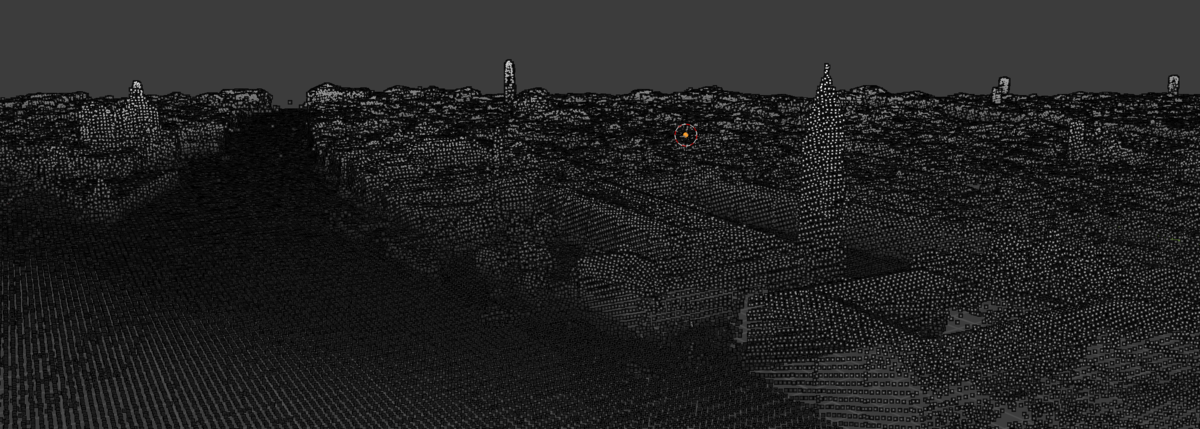
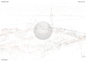
Point cloud denotes a 3D content representation which is commonly preferred due to its high efficiency and relatively low complexity in the acquisition, storage, and rendering of 3D models. In order to generate Venice dense point cloud models, sequential images from different angles in different locations need to be collected first based on the following two sources.
Youtube Video Method
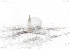
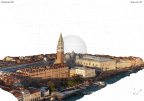
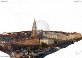
Our initial plan was to download drone videos of Venice on the Youtube platform, used FFmpeg to extract images from the video one frame per second, and generate dense point cloud models based on the images that we acquired. However, the videos we could get from drone videos are very limited: only a few of the videos are of high quality. Among those qualified videos, most videos only focused on monumental architecture such as St Mark's Square, St. Mark's Basilica, and Doge's Palace, where other buildings have a different extent of deficiencies from various angles in the point clouds. Therefore, a large proportion of Venice could not be 3D reconstructed if we only adopt Youtube Video Method.
Google Earth Method
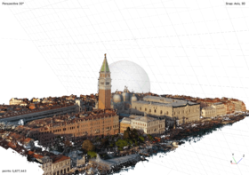
In order to access the comprehensive area of Venice, we decided to use Google Earth as a complementary tool: we could obtain images of every building we want at each angle. With Google Earth, we are able to have much more access to aerial images of Venice, not only will these images serve as images set to generate dense point cloud models in order to calculate building heights, but we can also use the overlapping part in different point cloud models to evaluate point cloud models in a cross-comparison way.
In a nutshell, we apply a photogrammetric reconstruction tool to generate point cloud models. Photogrammetry is the art and science of extracting 3D information from photographs. As for the Youtube-based method, we will only target famous buildings which appear in different drone videos and select suitable images to form the specific building's image set. With regard to the Google Earth method, we will obtain images of the whole of Venice manually in a scientific trajectory of the photogrammetry route.
Point Cloud Optimization
Outlier Removal
When collecting data from scanning devices, the resulting point cloud tends to contain noise and artifacts that one would like to remove. Apart from selecting points in Agisoft Metashape manually, we also use Open3D to deal with the noises and artefacts. In the Open3D, there are two ways to detect the outliers and remove them: statistical outlier removal and radius outlier removal. Radius outlier removal removes points that have few neighbors in a given sphere around them, and statistical outlier removal removes points that are further away from their neighbors compared to the average for the point cloud. We set the number of the neighbors to be 50, radius to be 0.01. Automatic outlier removal could remove around 75% percent of noise, but the effect isn't perfect, which is not as good as the manually gradual selection. Therefore, Automatic outlier removal could serve as a prepossessing step for the final de-noise, after automatic outlier removal, we still need to manually de-noise the point cloud.
Error Reduction
The first phase of error reduction is to remove points that are the consequence of poor camera geometry. Reconstruction uncertainty is a numerical representation of the uncertainty in the position of a tie point based on the geometric relationship of the cameras from which that point was projected or triangulated, which is the ratio between the largest and smallest semi axis of the error ellipse created when triangulating 3D point coordinates between two images. Points constructed from image locations that are too close to each other have a low base-to-height ratio and high uncertainty. Removing these points does not affect the accuracy of optimization but reduces the noise in the point cloud and prevents points with large uncertainty in the z-axis from influencing other points with good geometry or being incorrectly removed in the reprojection error step. A reconstruction uncertainty of 10, which can be selected with the gradual selection filter and set to this value or level, is roughly equivalent to a good base-to-height ratio of 1:2.3 , whereas 15 is roughly equivalent to a marginally acceptable base-to-height ratio of 1:5.5. The reconstruction uncertainty selection procedures are repeated two times to reduce the reconstruction uncertainty toward 10 without having to delete more than 50 percent of the tie points each time.
The second phase of error reduction phase removes points based on projection accuracy. Projection accuracy is essentially a representation of the precision with which the tie point can be known given the size of the key points that intersect to create it. The key point size is the standard deviation value of the Gaussian blur at the scale at which the key point was found. The smaller the mean key point value, the smaller the standard deviation and the more precisely located the key point is in the image. The highest accuracy points are assigned to level 1 and are weighted based on the relative size of the pixels. A tie point assigned to level 2 has twice as much projection inaccuracy as level 1. The projection accuracy selection procedure is repeated without having to delete more than 50% of the points each time until level 2 is reached and there are few points selected.
The final phase of error reduction phase is removing points based on reprojection error. This is a measure of the error between a 3D point's original location on the image and the location of the point when it is projected back to each image used to estimate its position. Error-values are normalized based on key point size. High reprojection error usually indicates poor localization accuracy of the corresponding point projections at the point matching step. Reprojection error can be reduced by iteratively selecting and deleting points, then optimizing until the unweighted RMS reprojection error is between 0.13 and 0.18 which means that there is 95% confidence that the remaining points meet the estimated error.[1]
Plane Generation
To calculate the height of the building, we have to find the ground of the Venice PointCloud model, which could be retrieved by a tool provided by Open3D. Open3D supports segmentation of geometric primitives from point clouds using "Random Sample Consensus", which is an iterative method to estimate parameters of a mathematical model from a set of observed data that contains outliers when outliers are to be accorded no influence on the values of the estimates. To find the ground plane with the largest support in the point cloud, we use segment_plane by specifying "distance_threshold". The support of a hypothesised plane is the set of all 3D points whose distance from that plane is at most some threshold (e.g. 10 cm). After each run of the RANSAC algorithm, the plane that had the largest support is chosen. All the points supporting that plane may be used to refine the plane equation, which is more robust than just using the neighbouring points by performing PCA or linear regression on the support set.
Plane Redressing
After selecting the most convenient plane and its supporting points, we define the plane equation in the 3D space. We want to build a PointCloud model where the Z coordinate of a point equals the height of this point in real world, so the next step is to redress the plane by projecting it on an X-O-Y space. For the projection calculation, we used the projection matrix mentioned below.
Here, the plane equation is ax + by + cz + d = 0 The redressing was performed in two steps, first translation and then rotation.
For translation, the plane intersects Z-axis at (0, 0, -d/c). So the translation is
which passes through the origin and vector v = (a, b, c)T
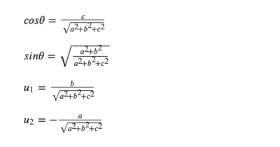
For the rotation, the angle between v and k = (0, 0, 1)T' is given by:
The axis of rotation has to be orthogonal to v and k. so its versor is:
The rotation is represented by the matrix:
Please note that:
Height Visualisation
Point-to-Plane Based Height Calculation and City Elevation Model Construction
Once the plane equation is obtained in the previous step, we could start calculating the height of buildings. In the first step, we calculate the relative height of the buildings based on the formula of point-to-plane distance. The coordinate information of each point could be accessed by the 'points' attribute of the ‘PointCloud’ object with the help of 'Open3D'. Since we already have the plane equation, using this formula, we could obtain the distances between each point and the plane and save them in a (n, 1) array.
To visualise the height of the building, the first method is to change the colors of the points in the PointCloud model. For each point in the ‘PointCloud’, it has a ‘Colors' attribute. By calling this attribute, an (n, 3) array of value range [0, 1], containing RGB colors information of the points will be returned. Therefore, by normalising the ‘distances array’ values to the range of [0,1] and expanding the 'distances array' to three dimensions by replication, we get a (n, 3) ‘height array' in the form of (n, 3) 'colors array’.
Basically, we transform the height information of each point to its 'colors' information, expressing the height by its color, higher points have lighter colors and vice versa. This model provides us with an intuitive sense of the building heights, which is more qualitative than quantitative.
Coordinate Based Height Calculation and City Elevation Map Construction
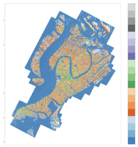
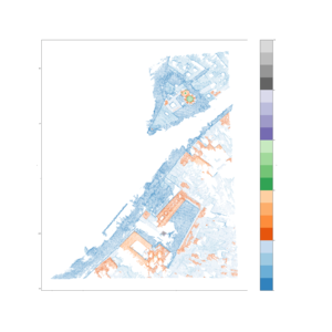
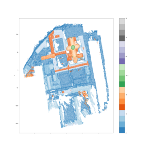
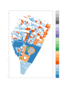
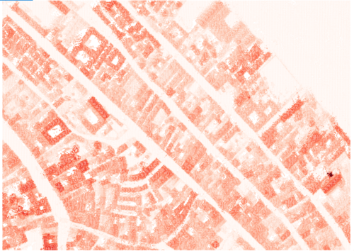
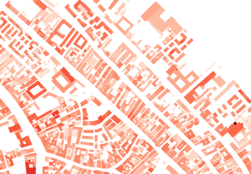
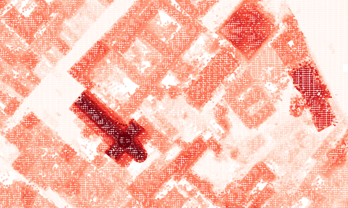
To show the building heights more quantitatively, we decided to construct a City Elevation Map, which could be achieved by plotting the height information of points in a 2D map. However, there is a prerequisite: we should get the actual height information of every point. After implementing "Plane Redressing", we assume that the z-coordinate can be approximated as the height. But before directly using it, we still need to scale the model so that the height of buildings in the model matches the actual height of buildings. For instance, we know the actual height of a reference point in the real world, and we could also obtain the height of this reference point in the PointCloud model, therefore, we could obtain the scale factor in this PointCloud model. For all the other buildings in the model, the actual height equals the height in the PointCloud model multiplying the scale factor.
To put it into practice, we need to set a reference point in the model, "Campanile di San Marco" is the best choice. The height of the highest building in Venice, "Campanile di San Marco", is 98.6 metres. In this step, the built-in function "Scale" from Open3D is adopted, and we finally obtained a 1:1 Venice PointCloud model where the z-coordinate of a point equals the actual height of this point in the real world.
To get the HD version of the City Elevation Map, please check xxx.
Cadaster Alignment
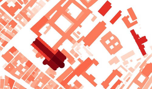
In order to map our City Elevation Map to the cadaster map, we use QGIS for georeferencing[1], which is the process of assigning locations to geographical objects within a geographic frame of reference. QGIS enables us to manually mark ground control points in both maps: Firstly, we select a representative location from the city elevation map, then we select the same location in the reference cadastre map. We set around ten pairs of ground control points to align the two maps, and the Venice zone EPSG 3004 should be chosen as the coordinate reference system when it comes to the transformation setting. The blue layer is the cadaster map while the red layer is our city elevation map. The georeferencing result is acceptable, where our height map matches the cadaster mostly accurately without distortion.
Quality Assessment
To assess the precision of our model, we compared the
What is left to be done: 1. Write description of assessment method 2. Calculate the error 3. add pictures
Objective Assessment of Google-Earth-Based Venice Model
Assessment of Landmarks
| Name of Buildings | Average Measured Height | Reference Height | Error Percentage | Picture |
|---|---|---|---|---|
| Basilica di San Marco | 44m | 43m | 2.32 | |
| Campanile di San Marco | 99m | 98.6m | 0.40 | |
| Chiesa di San Giorgio Maggiore | 42m | NA | ||
| Campanile di San Giorgio Maggiore | 72m | 63m | 12.5 | |
| Basilica di Santa Maria della Salute | 64m | NA | ||
| Campanile di Santa Maria della Salute | 49m | NA | ||
| Basilica dei Santi Giovanni e Paolo | 54m | 55.4m | 2.52 | |
| Campanile di Chiesa di San Geremia | 50m | 50m | 0.00 | |
| Campanile dei Gesuiti | 43m | 40m | 7.5 | |
| Campanile San Francesco della Vigna | 76m | 69m | 10.14 | |
| Chiesa del Santissimo Redentore | 47m | 45m | 4.44 | |
| Hilton Molino Stucky Venice | 45m | NA |
Assessment of other Buildings
| Buildings near Basilica dei Santi Giovanni e Paolo | Buildings near Basilica dei Frari | ||||||
|---|---|---|---|---|---|---|---|
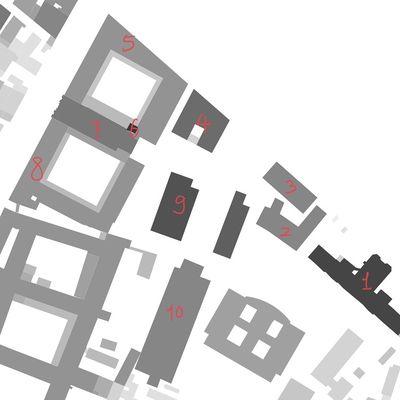
| Index | Average Measure Height | Reference Height | Error Percentage | Index | Average Measure Height | Reference Height | Error |
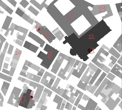
| 1 | 28.25m | 28.1m | 0.53 | 11 | 63m | 63.07 | 0.11 |
| 2 | 19.5m | 19.44m | 0.03 | 12 | 31m | 30.94 | 0.19 |
| 3 | 18.5m | 18.77m | 1.43 | 13 | 20m | 20.8m | 3.84 |
| 4 | 23m | 22.59m | 1.81 | 14 | 20m | 21.28 | 6.01 |
| 5 | 17m | 16.95m | 0.29 | 15 | 26m | 28.22m | 7.86 |
| 6 | 31m | 30.83m | 0.55 | 16 | 24m | 24.92m | 3.69 |
| 7 | 20.5m | 21.02m | 2.47 | 17 | 26m | 26.4m | 1.51 |
| 8 | 17m | 17.24m | 1.39 | 18 | 46m | 46.58m | 1.24 |
| 9 | 27.5m | 26.31m | 4.52 | 19 | 15m | 15.87m | 5.48 |
| 10 | 19.5m | 19.41m | 0.46 | 20 | 10m | 10.56m | 5.30 |
Objective Assessment of Youtube-Video-Based Venice Model
| Buildings near Basilica Cattedrale Patriarcale di San Marco | Buildings near Basilica di Santa Maria della Salute | ||||||
|---|---|---|---|---|---|---|---|
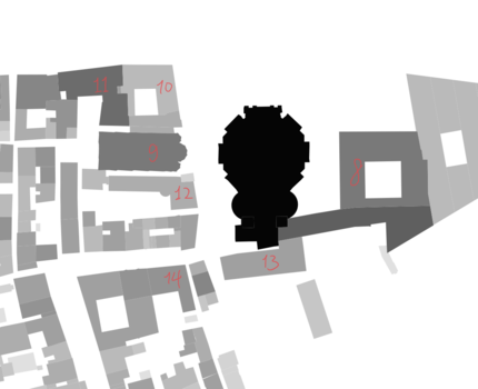
| Index | Average Measure Height | Reference Height | Error | Index | Average Measure Height | Reference Height | Error |
| 1 | 99m | 98.6m | 0.40 | 8 | 21m | 21.76m | 3.49 |
| 2 | 44m | 43m | 2.32 | 9 | 19m | 20.12m | 5.56 |
| 3 | 30m | 30.59m | 1.92 | 10 | 11m | 11.15m | 1.34 |
| 4 | 24.33m | 23.21m | 4.82 | 11 | 22m | 23.21m | 5.21 |
| 5 | 26m | 26.35m | 1.32 | 12 | 11m | 12.07m | 8.86 |
| 6 | 21m | 22.21m | 5.44 | 13 | 14m | 14.18m | 1.26 |
| 7 | 21m | 21.53m | 2.46 | 14 | 16m | 16.98m | 5.77 |
Subjective Assessment
During the subjective assessment, We gather ten volunteers to give their subjective scores on our part of Digital Elevation map. Here we use Double Stimulus Impairment Scale (DSIS) which is a type of double stimulus subjective experiment in which pairs of images are shown next to each other to a group of people for the rating. One stimulus is always the reference image, while the other is the image that needs to be evaluated. The participants are asked to rate the images according to a five-levels grading scale according to the impairment that they are able to perceive between the two images (5-Imperceptible, 4-Perceptible but not annoying, 3-Slightly annoying, 2-Annoying, 1-Very annoying). We will compute the Differential Mean Opinion Score (DMOS). The DMOS score can be computed as:
where N is the number of subjects and DVij is the differential score by subject i for the stimulus j.
The two detailed reference maps are always set to be 5.The DMOS score of the both images below
Display of YouTube-Video-Based Venice Models
Basilica Cattedrale Patriarcale di San Marco
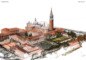
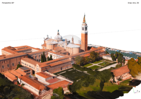
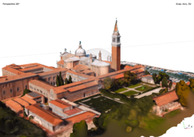
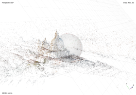
Basilica di San Giorgio Maggiore
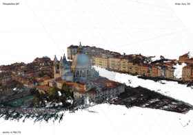
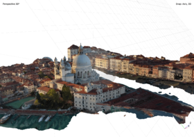
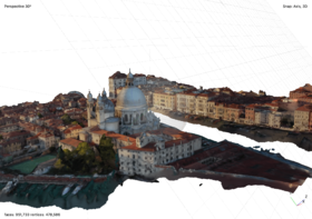
Basilica di Santa Maria della Salute
Limitations and Further Work
Limitations
- Challenges in model implementation from Google Earth Image
Using Google Earth images is a solution to the problems mentioned above. But it is not a perfect method either. It seemed that we were in a dilemma when we tried to collect images from Google Earth: When we took screenshots from a long distance from the ground, the resolution of images was very low, the details of the buildings were not well rendered, thus causing the low quality of the PointCloud model. When we took screenshots from a short distance from the ground, we obtained a much better result, the details were much clearer. But to get this result, the number of images we needed to build the PointCloud model increase exponentially, and the calculation was almost impossible for a Personal Computer to afford.
One possible solution is dividing Venice into smaller parts, building a PointCloud for every part, and merging the PointClouds models together in the end. However, this solution requires registration, which is not only quite imprecise, but also hard to implement.
- Inaccurate Plane Generation and Redressing
One of the inherent defects in the methodology is 'Plane Generation' and 'Plane Redressing' are imperfect. When we implement 'Plane Redressing', the ideal scenario is that after a single transformation, the plane equation would become 0x + 0y + z = 0. However, when we implement the transformation, it is not the case: the coefficients before x and y are not exactly 0. The error caused by this inherent defect could be neutralised by implementing the transformation for 1000 times: When the number of iterations increases, the coefficients before x and y approaches zero infinitely.
Further Work
- More Precise Georeferencing and Pixel Matching
We only choose ten ground control points for QGIS to georeference the raster height map. Generally, The more points you select, the more accurate the image is registered to the target coordinates of the cadaster. In the future, after choosing enough ground control points, we will compare our Venice elevation map with the cadaster pixel by pixel in the same resolution. Both maps use the same color and grey scales.
- Building Contour Sharpening
In our Venice elevation map, the building footprint is blurred and not well detected. In the future, we will use Shapely in Python to find the polygons and OpenCV to implement contour approximation.
References
[1] https://pubs.er.usgs.gov/publication/ofr20211039
Deliverables
- Source Codes: https://github.com/yetiiil/venice_building_height
- Venice Point Cloud Models:


