Tracking a Historic Market Crash through Articles
Introduction and Motivation
The impact of economic crises on the socio-economic fabric of society is immense, with widespread and far-reaching effects on social stability and people's standard of living, as they can cause markets to shrink, businesses to lose capacity and unemployment to soar. While the recovery period from economic crises can span several years and the economic damage can be comparable to that of a major natural disaster, we recognize that predicting the emergence of economic crises with complete accuracy is a challenging goal. We therefore turn to the potential link between financial newspapers and the early warning signs of economic crises. While we cannot expect to flawlessly predict crises through the news media, we believe that by analyzing textual data from financial newspapers, we can reveal some early signs of market trends that could be useful in mitigating the losses that individuals, businesses, and countries may suffer during economic crises.
The news media, as one of the main channels of information for the public, not only reflects the current economic situation, but also plays a crucial role in shaping the public perception of the economic situation. Therefore, the news media is not only a recorder of the economy, but the information it conveys may also influence the future direction of the economy.
As the world's largest economy, the economic dynamics of the United States have far-reaching implications for global markets. The global financial crisis of 2008, which began in the United States and quickly spread across the globe, had far-reaching consequences and lessons learned. The data from this period provide a valuable opportunity to study the patterns of major economic crises and crisis warning signals. In addition, compared with new media, traditional media are more authoritative and reliable, and can more faithfully reflect the economic conditions and public perceptions of the economic situation at the time. Therefore, we chose data on U.S. economic indicators from 2006 to 2013 as well as news reports from Bloomberg as our research dataset.
The goal of our research is to construct an accurate prediction model that extracts features from text data of news papers to predict changes in economic indicators. Through this prediction model, we expect to warn of major economic crises in advance and assist governments, enterprises and individuals to take early measures to mitigate the significant impacts of economic crises in order to protect the country, society and individuals from serious losses.
Methodology
Data Collection
News dataset
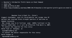
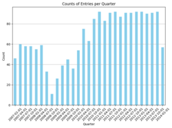
Bloomberg Businessweek is an economic and business-oriented weekly magazine published by Bloomberg, a global multimedia corporation. Renowned for its in-depth coverage, analysis, and commentary on global business, finance, technology, markets, and economics, this publication offers a comprehensive view of various industry trends, corporate strategies, and market dynamics. The dataset is generated from Bloomberg website through their public APIs by Philippe Remy and Xiao Ding. It contains 450,341 news from 2006 to 2013.
Predictive indicators
fredaccount.stlouisfed.org is affiliated with the Federal Reserve Bank of St. Louis and is part of its FRED (Federal Reserve Economic Data) system.FRED provides a wide range of economic data, including data from different sources. Users can find, download, plot and track economic data for various periods and regions on this site. Overall, fredaccount.stlouisfed.org is a valuable resource for anyone interested in researching and analyzing the economic situation. We looked up key economic indicators for the U.S. from 2006-2013.
Monthly indicators including:
- Employment Level
- Industrial Production Total Index (INDPRO)
- Manufacturing and trade Industries Sales (CMRMT)
Quarterly indicators including:
- Real Gross Domestic Product
- GDP Growth Rates
Data Preprocessing
Text Data Cleaning
Textual data undergoes a rigorous cleaning process as the initial step. This involves the elimination of numerical digits, special characters, and punctuation marks from the text. This meticulous cleansing enhances the readability and suitability of the text for subsequent analyses.
Text Tokenization and Lemmatization
Post-cleaning, the text is subjected to tokenization and lemmatization. Tokenization disassembles the text into individual words or tokens, while lemmatization reduces these tokens to their base or root forms. This standardization minimizes the impact of varying word forms on analytical outcomes.
Stopwords Removal
The process of removing stopwords involves the exclusion of frequently occurring words that contribute minimal semantic value to the analysis. This includes a carefully curated set of stopwords, incorporating additional stopwords provided by citations2. By eliminating these extraneous words, the noise within the text is mitigated, resulting in more accurate analysis.
Feature Extraction
TF-IDF
TF-IDF, an abbreviation for Term Frequency-Inverse Document Frequency, holds a pivotal role in the domain of text mining. It stands as a cornerstone technique for determining the significance of terms within a collection of documents. It relies on two fundamental principles: Term Frequency (TF) and Inverse Document Frequency (IDF).
- Term Frequency (TF) quantifies how often a term appears within an individual document. A term's frequency is higher when it occurs more frequently within a document.
- Inverse Document Frequency (IDF) encapsulates the significance of a term across the entire document corpus. It computes the reciprocal of a term's frequency across all documents, distinguishing common yet less consequential terms from those of higher corpus-specific importance.
The computation of TF-IDF involves multiplying TF by IDF, amalgamating a term's local significance within a single document with its global significance across the entire corpus.
In our research endeavors, the application of TF-IDF enables the evaluation of the significance of selected financial terms within individual articles. This methodology facilitates the identification of pivotal terms (a) within specific articles (w), prioritizing their contextual relevance over their frequency within the entire corpus. Furthermore, our approach avoids information leakage by utilizing daily occurrence counts of terms, ensuring the accuracy and reliability of our analytical processes. The frequency of the term in each article is defined as tf(a)_w, the number of articles per day N_t, and the number of articles in which the term appears per day n_t < N_t. The tf-idf function could be defined as:
Transformer Models
DistilBERT
DistilBERT is characterized by its smaller size and faster processing capabilities compared to its predecessor, BERT. It retains a significant majority of the original model's language understanding power. The model is optimized for performance and efficiency, designed to be cost-effective for training while still delivering robust NLP capabilities. The training foundation for DistilBERT is the same as BERT's, using the same pre-training datasets which typically include large corpora such as BooksCorpus and English Wikipedia.
Twitter-roBERTa
This model(Twitter-roBERTa) is a variant of the roBERTa-base that has been trained on approximately 58 million tweets and fine-tuned for sentiment analysis. It is designed to classify sentiments expressed in tweets into negative, neutral, or positive categories. The model's training used the TweetEval benchmark and is tailored for English language tweets. This model is especially useful for analyzing social media content where expressing sentiments succinctly is common.
FinBERT
FinBERT is a BERT model pre-trained on a wide range of financial texts to enhance financial NLP research and practice. It is trained on corporate reports, earnings call transcripts, and analyst reports, totaling 4.9 billion tokens. This model is particularly effective for financial sentiment analysis, a complex task given the specialized language and nuanced expressions used in the financial domain.
FinBERT-Tone
This model(FinBERT-Tone) is a fine-tuned version of FinBERT specifically for analyzing the tone of financial texts. It has been adjusted on 10,000 manually annotated sentences from analyst reports, labeled as positive, negative, or neutral. The model excels in financial tone analysis tasks and is an excellent choice for those looking to extract nuanced sentiment information from financial documents.
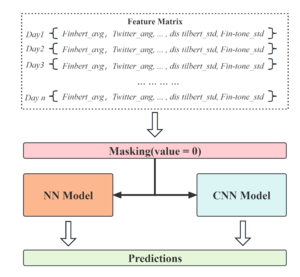
After obtaining the sentiment scores for each news text, we aggregated the sentiment scores on a day-by-day basis. The mean and variance of the sentiment scores for the day predicted by the four pre-trained models were calculated and saved separately. Based on the assumption that neutral articles do not significantly affect people's perceptions, we did not include neutral (i.e., news with a sentiment score of 0) in the calculation of sentiment score statistics. For missing dates, we used zero-padding and ignored missing values in conjunction with a masking mechanism in deep learning.
Machine Learning Models for Prediction
Model Introduction
Given the timestamped nature of the news text, our primary focus revolves around managing time series data. To tackle TF-IDF and sentiment analysis, we've adopted distinct prediction models. While exploring a spectrum of machine learning models and neural networks, we've meticulously filtered and retained the top-performing trio for each segment based on their efficacy within our dataset.
For TF-IDF, our selection comprises the GradientBoosting Regressor, Multi-Layer Perceptron Regressor (MLP), and Random Forest Regressor. In the realm of sentiment analysis, we've opted for the Random Forest, Neural Networks, and Convolutional Neural Networks (CNN).
GradientBoosting Regressor
The GradientBoosting Regressor is an ensemble learning method used for regression tasks. It builds a strong predictive model by combining multiple weaker models, usually decision trees, sequentially. It works by fitting each new model to the residuals (the difference between predicted and actual values) of the preceding model, gradually improving predictions. This iterative process focuses on reducing errors, enhancing model performance. GradientBoosting Regressor is adept at handling complex relationships in data and tends to provide more accurate predictions than individual models.
Multi-Layer Perceptron Regressor(MLP)
MLP is an artificial neural network designed for regression tasks. It comprises interconnected layers of nodes processing inputs through nonlinear activation functions. This model excels in capturing intricate patterns in data, ideal for complex regression problems. During training, it adjusts weights between nodes to minimize errors using forward and backward propagation. However, its performance hinges on hyperparameters like layer depth, node count, and learning rate, demanding careful tuning.
Random Forest Regressor
The Random Forest Regressor constructs multiple decision trees during training and aggregates their predictions to provide a regression outcome. By combining predictions from diverse trees, it minimizes overfitting and variance while improving accuracy in regression tasks. This technique utilizes randomness in both data sampling and feature selection, making it robust against noise and suitable for handling complex datasets with numerous input variables. Its ability to handle non-linear relationships and maintain predictive performance makes it a popular choice in regression analysis.
Random Forest
Random Forest is an integrated learning technique that is an extension of the decision tree model. Random Forest will improve prediction accuracy by training multiple decision trees and combining the results of multiple decision trees. Since each decision tree is trained on a different subset of data, Random Forest is more robust to noise and overfitting.
Neural Networks (NN)
Neural Networks (NN) is a computing system that mimics the structure and function of the human brain to process complex data sets. It consists of multiple layers of nodes, each of which can receive, process and transmit information. Neural networks typically learn through a back-propagation algorithm that continuously adjusts the connection weights between nodes to best represent the characteristics of the input data. This learning ability allows neural networks to excel in tasks such as image recognition, natural language processing, and predictive modeling. The design and functional diversity of neural networks makes them a central component of artificial intelligence and machine learning research.
CNN
Convolutional Neural Networks (CNNs) are a powerful tool in the field of deep learning and were first used for image recognition. In recent years, they have also been applied to time-series data analysis. In time-series analysis, CNNs can effectively capture local features and temporal dependencies in data. By using a convolutional layer, CNNs can process input sequences of different lengths to recognize patterns in data of different time intervals. The core advantage of temporal convolution is its ability to effectively extract time-dependent features while maintaining the order of the time series, which is crucial for prediction tasks.
Training Settings
Data Setting
Matching news features with economic indicators using a sliding time window, considering different lengths of the time series, with 31 and 92 days as the maximum number of days in a month and quarter, and missing dates are filled with zeros using post-padding.
Model Construction
- RF: One-dimensional spreading of the feature matrix is performed as input and max_features is set to 'sqrt' to allow the decision tree to continue to grow when the minimum branching condition is satisfied.
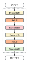
- NN: A double hidden layer structure incorporating BatchNormalization was designed to perform regression analysis using a linear activation function designed to capture the complex relationship between news text and economic indicators.
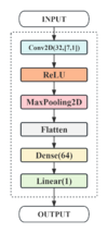
- CNN: A convolutional kernel of size (n,1) is applied to design time-series convolutional layers of different sizes for monthly and quarterly metrics in order to extract features at different time scales.
- MLP: An MLP architecture featuring two hidden layers integrated with BatchNormalization was crafted for regression analysis. It utilizes a linear activation function, tailored to comprehend the intricate correlations between news text and economic indicators.
Model Training
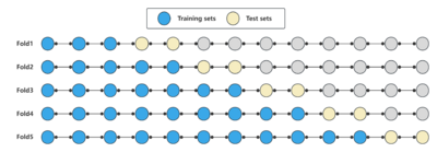
Cross-validation: Given the unsuitability of regular cross-validation for time series data, we adopt a time window approach for conducting 5-fold cross-validation. This method evaluates the model's performance at various time points through time-series cross-validation, ensuring the retention of complete historical data to maintain stability in the length of the training sequence.
Masking Mechanism: In the sentiment analysis task, a masking mechanism was introduced to handle sparse data due to time windows, while regularization and early stopping were applied to mitigate overfitting.
Model Parameter Setting
| Basic structure | Optimization (optimizer, loss function) | Training details | |
|---|---|---|---|
| RF |
|
HRNetV2p-W18-Small |
|
| NN |
|
Adam(lr = 0.001) loss='mean square error' |
|
| CNN |
|
Adam(lr = 0.001) loss='mean square error' |
|
Model Integration
Results and Quality Assessments
Assessment
TF-IDF
In the comprehensive evaluation of model fitting, we considered various metrics, particularly focusing on the predictive performance concerning small-scale datasets. MSE, MAE, MAPE, and R2 were chosen as our evaluation benchmarks to gain a holistic understanding of the model's performance across different facets. To ensure the model's interpretability and prevent overfitting, we employed R2 as the loss function during the grid search for TF-IDF hyperparameter tuning. During the testing phase, we integrated these four metrics to provide a comprehensive assessment of the model's performance.
Sentiment Analysis
When training for deep learning, we examine three different loss functions. In the calculation of MSE, larger errors are penalized more heavily as they are squared, thus making the model more sensitive to outliers; furthermore, assuming that the errors satisfy a Gaussian distribution, MSE conforms to the maximum likelihood estimation of the Gaussian distribution that minimizes the errors. Because of MSE's sensitivity to large errors and optimization friendliness, we chose the most suitable MSE loss function for model training.
The following is a description of the assessment indicators:
Mean Squared Error (MSE) is a statistical measure used to evaluate the accuracy of a predictive model. It calculates the average of the squares of the differences between predicted and actual values. The squaring ensures that errors are positive and emphasizes larger errors more than smaller ones. A lower MSE value indicates a model with better predictive accuracy.
Mean Absolute Error (MAE)is a metric used to measure the average magnitude of errors between predicted and actual values in a dataset. To calculate MAE, you first find the absolute differences between predicted and actual values for each data point, then take the average of these absolute differences. In machine learning and statistical modeling, MAE serves as a common evaluation metric to assess the performance of models. A smaller MAE indicates better accuracy in predictions.
Mean Absolute Percentage Error(MAPE)measures the average percentage difference between predicted and actual values. It has an advantage on small-scale datasets such as CAGR as it represents errors in percentage terms, providing a clearer reflection of relative errors regardless of the data's scale. This makes it useful for comparisons across different scales as it offers a consistent measure unaffected by data magnitude.
Coefficient of Determination(R^2)is a metric used to assess the goodness of fit of a regression model. It represents the proportion of variance in the dependent variable that is predictable from the independent variables. This score ranges from 0 to 1.
In particular, given that we have multiple economic indicators, we need to evaluate the performance of the models in a comprehensive manner.
For each model, we performed at least 5 repetitions of the experiment. The reproducibility of the model is ensured by setting random seed. The average of the five experiments was taken as the final performance evaluation of the model. The results of the repeated experiments can be accessed in the Deliverables.
Results
Prediction results based on TF-IDF
GDP
| Model | Parameters |
|---|---|
| LinearRegression | - |
| SVR | Kernel: linear, C = 0.1, gamma = 0.1 |
| DecisionTreeRegressor | Criterion: poisson, Max Depth: 5, Min Samples Split: 2 |
| RandomForestRegressor | n_estimators: 50, Max Depth: 5, Min Samples Split: 2 |
| GradientBoostingRegressor | Learning Rate: 0.1, Max Depth: 5, n_estimators: 150 |
| MLPRegressor | Hidden Layer Sizes: (100, 50), Max Iterations: 500, Solver: lbfgs, Activation: relu, Alpha: 0.001, Learning Rate: invscaling |
| Model | Training R^2 | Testing R^2 | Training MAE | Testing MAE | Training MSE | Testing MSE | Training MAPE | Testing MAPE |
|---|---|---|---|---|---|---|---|---|
| LinearRegression | 1.000 | -0.015 | 3.1225e-18 | 0.000977 | 3.6111e-35 | 1.1579e-06 | 7.2536e-15 | 2.3569 |
| SVR | -0.0037 | -0.4666 | 0.001256 | 0.001166 | 2.0851e-06 | 1.6724e-06 | 2.9814 | 2.8152 |
| DecisionTreeRegressor | 0.9999 | 0.3348 | 3.0562e-06 | 0.000686 | 9.3404e-11 | 7.5851e-07 | 0.0073 | 1.6437 |
| RandomForestRegressor | 0.9728 | 0.6601 | 0.000186 | 0.000556 | 5.6504e-08 | 3.8764e-07 | 0.4451 | 1.3344 |
| GradientBoostingRegressor | 1.000 | 0.6123 | 9.9113e-09 | 0.000518 | 2.1313e-16 | 4.4212e-07 | 0.000023 | 1.2349 |
| MLPRegressor | 0.2067 | -1492.5717 | 0.000911 | 0.0348 | 1.6479e-06 | 1.7031e-03 | 2.1859 | 83.9713 |
PAYEMS
| Model | Parameters |
|---|---|
| LinearRegression | - |
| SVR | Kernel: linear, C = 10, gamma = 0.1 |
| DecisionTreeRegressor | Criterion: absolute_error, Max Depth: 10, Min Samples Split: 5 |
| RandomForestRegressor | n_estimators: 50, Max Depth: 10, Min Samples Split: 2 |
| GradientBoostingRegressor | Learning Rate: 0.1, Max Depth: 3, n_estimators: 150 |
| MLPRegressor | Hidden Layer Sizes: (100, 50), Max Iterations: 500, Solver: lbfgs, Activation: relu, Alpha: 0.001, Learning Rate: invscaling |
INDPRO
| Model | Parameters |
|---|---|
| LinearRegression | - |
| SVR | Kernel: linear, C = 10, gamma = 0.1 |
| DecisionTreeRegressor | Criterion: absolute_error, Max Depth: 10, Min Samples Split: 2 |
| RandomForestRegressor | n_estimators: 100, Max Depth: 10, Min Samples Split: 2 |
| GradientBoostingRegressor | Learning Rate: 0.1, Max Depth: 3, n_estimators: 150 |
| MLPRegressor | Hidden Layer Sizes: (100, 50), Max Iterations: 500, Solver: lbfgs, Activation: relu, Alpha: 0.001, Learning Rate: invscaling |
CMRMT
| Model | Parameters |
|---|---|
| LinearRegression | - |
| SVR | Kernel: poly, C = 0.1, gamma: auto |
| DecisionTreeRegressor | Criterion: absolute_error, Max Depth: 15, Min Samples Split: 2 |
| RandomForestRegressor | n_estimators: 100, Max Depth: 10, Min Samples Split: 5 |
| GradientBoostingRegressor | Learning Rate: 0.1, Max Depth: 3, n_estimators: 150 |
| MLPRegressor | Hidden Layer Sizes: (100, 50), Max Iterations: 500, Solver: lbfgs, Activation: relu, Alpha: 0.001, Learning Rate: invscaling |
Prediction results based on sentiment score
In evaluating the INTRO metrics, we explored various model and parameter configurations with and without masking (masking). After a series of experiments, we conclude that CNN-2 performs best under these conditions. Based on this finding, we believe we have found an effective model adapted to the current demand for forecasting time series data.
| Hyperparameters | Label | Loss Test | MSE_all | |
|---|---|---|---|---|
| CNN-1 | Default | INDPRO | mean_squared_error | 0.0458 |
| CNN-2 | Masking | INDPRO | mean_squared_error | 0.0296 |
| NN-1 | Default | INDPRO | mean_squared_error | 0.1097 |
| NN-2 | Masking | INDPRO | mean_squared_error | 0.097 |
| RF-1 | Default | INDPRO | MSE,RMSE,R2 | MSE: 0.1062, RMSE: 0.3258, R2: -0.0737 |
| RF-2 | Masking | INDPRO | MSE,RMSE,R2 | MSE: 0.1052, RMSE: 0.3244, R2: -0.0642 |
After obtaining the optimal model, we tested it on several labels and got good results, which confirmed the strong generalization ability of the model.
| Experiment number | Label | Loss | |
|---|---|---|---|
| CNN-2 | 1 | CMRMT | loss: 0.0107 - val_loss: 0.0296 |
| CNN-2 | 2 | Employment Level | loss: 0.0168 - val_loss: 0.0816
|
| CNN-2 | 3 | INDPRO | loss: 0.0102 - val_loss: 0.0642 |
| CNN-2 | 4 | RGDP | loss: 0.0165 - val_loss: 0.0234 |
| CNN-2 | 5 | CAGR2 | loss0.0130 - val_loss 0.0663 |
Prediction results of Integration
Limitations
Feature engineering
We only calculated the statistics and TF-IDF matrix of the sentiment scores of the news text, without fully considering all the features of the news text. Although deep learning models are able to automatically learn deep features of the data from the input, more optimal feature engineering, such as named entity recognition or topic analysis, may still be beneficial for model training.
Overfitting
Although we imposed regularization and early stopping to mitigate overfitting, we are still unable to effectively avoid overfitting due to the small dataset. It is also evident from the model's prediction results that the training set is significantly better than the test set. The results of the time-series cross-validation show that the performance of the model gradually.
Future Work
1. Expanding the dataset
In order to improve the generalization ability and accuracy of the model, a key direction for future work is to expand the existing dataset. This includes collecting more diverse data samples, such as news texts and economic indicator data from different regions and eras.
2. Feature Expansion and Feature Fusion
Feature engineering involves exploring new feature sets as well as investigating potential associations between existing features. In addition, the optimization of feature fusion strategy is also an important research point. Our current strategy is to perform decision fusion for different models, and the limited feature dimensions may limit the learning ability of the model. Feature fusion involves how to effectively combine features from different sources and types to enhance the learning ability of the model.
3. Multimodal learning
The exploration of multimodal learning will be an important part of future work. Multimodal learning involves processing and analyzing data from different modalities (e.g., text and images) simultaneously. This approach provides a more comprehensive view of the data and enhances the model's ability to process complex and diverse data.
Project Plan and Milestones
Weekly Project Plan
| Week | Tasks | Completion |
|---|---|---|
| Week 4 |
|
✓ |
| Week 5 |
|
✓ |
| Week 6 |
|
✓ |
| Week 7 |
|
✓ |
| Weeks 8–9 |
|
✓ |
| Week 10 |
|
✓ |
| Week 11 |
|
✓ |
| Week 12 |
|
✓ |
| Week 13 |
|
✓ |
| Week 14 |
|
✓ |
Milestones
Milestone 1
- Draft a comprehensive project proposal outlining aims and objectives.
- Identify datasets with appropriate time granularity and relevant economic labels.
- Prepare and clean selected datasets for analysis.
Milestone 2
- Master the NLP processing workflow and techniques.
- Construct TF-IDF representation and emotional indicators in news data.
- Conduct preliminary model adjustments to enhance accuracy based on initial data.
Milestone 3
- Implement pre-trained models for sentiment analysis and integrate them into the project.
- Apply decision fusion techniques to optimize model performance.
- Refine and fine-tune the models based on the results and feedback.
Milestone 4
- Prepare the final presentation summarizing and visualizing the project findings and outcomes.
- Create and finalize content for the Wikipedia page, documenting the project.
- Conduct a thorough project review and ensure all documentation is complete and accurate.
Deliverables
Source codes and training recordings:[ ]
Datas:GoogleDrive
