Coal supply in the German Empire

Map of the Coal supply in the German Empire, in 1881.

Main ideas

• To study the coal supply and demand of the German Empire for the year 1881.
• Interactive visualization of Germany's main coal production and consumption centers.
• Dynamic visualization of coal transport flows according to the different mining basins and transport routes.
• Differentiating the production and consumption centers from the transport hubs.
• Inspiration for presenting the data: https://vimeo.com/250033884
• Creation of a website to present the results.
• Interpretation of the results: the role of coal in the German Unification (Macroeconomic aspects of German unification preceding the political unification).

Map details

• 

  Berlin as one on the main consumption center.

• 

  The Ruhr, Germany's main industrial center.

• 

  Bremen and Bremerhafen, a small consumption center, but a huge transport hub.

• 

  The extremely precise scale system.

• 

  Colors legend.

Historical introduction to the map

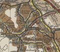
We are working on a historical map that originates from Germany and is dated from 1881. On this map of central and northern Europe, the German Empire is represented as it existed in the year 1881. The originality of the document is that it features the consumption, and the production of coal of many important German cities of the Empire, as well as the annual fluxes of coal being transported between cities by train or by boat. It was commissioned by the German Empire's Ministry of Public Works, authored by Simon Schropp and edited by Schropp (Berlin).

Large-scale coal mining developed during the Industrial Revolution and coal was the central source of energy for industry and transportation in industrial areas of 19th century Germany. The link between the two strategical assets that are coal production and railway deployment is reciprocal. Railway transportation system, because of their high coal consumption, influenced the development of coal production more than coal production influenced the development of the railway system, but the necessity to transport that ever-increasing amount of coal in order to feed the newly integrating German economic system and gain independence from British coal did boost the development of the railway network.

What is particularly interesting about that map is that the complex and interwoven network of coal production and transportation that it represents is happening only 10 years after the German unification. It confirms what secondary literature has already established: the economic union of Germany preceded the political union, the latter one being the culmination of the economic integration. It started with the formation of the Zollverein, the German customs union which allowed the easier transport of goods between the German states. But more importantly, the development of the rail technology and the states' investment in the corresponding rail network allowed the growth of a German-wide supply-chain.

The Union was a coalition of German states managing their tariffs and their economy as a unified economic territory. The Zollverein was launched on 1 January 1834. But in reality, its foundations started in 1818 with the creation of a variety of customs unions among the German states. By 1866, the Zollverein included most of the German states. The foundation of the Zollverein was the first instance in history in which independent states had created a full economic union without the simultaneous creation of a political federation. Politically, Prussia was the member state driving the creation of the customs union while Austria was excluded from the Zollverein because of its highly protected industry. After the unification of the German states in 1871, the Empire assumed control of the Zollverein. Indeed, the three main Prussian objectives in the development of the Zollverein were first, as a political tool to eliminate the excessive Austrian influence in Germany; second, as a way to improve their economy; and third, to strengthen the concept of a Prussian Germany against potential French aggression while reducing the economic independence of smaller states. The full political unification was the result but not the stated goal of the economic integration.

That same integration made the creation of a railway system necessary, while that system rendered the integration easier in a positive loop of economic and political harmonization. Before the Zollverein, the political infighting between conservative states made it a challenge to build railways in the 1830s but the growing importance of the Zollverein made the construction of a coherent infrastructure a possibility. By the middle of the 19th century, rail linked the major cities; each German state is responsible for the lines within its own borders.

Freight Cost

Until the 1820s, the nobility championed economically inefficient but prestigious canal projects over railways. In the 1830s, the growing liberal middle classes supported state-sponsored railways as a form of progress with direct benefits for the German people’s capacity to move around as well as for the shareholders in the joint stock companies that built and operated the railroads. Though private railway enterprises did exist, they were taken over by state companies in the 1840s. However, those state-owned enterprises copied many of the private companies' methods and organizational structures.

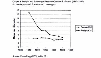
The complex links between political goals and economic objectives are made clearer by the fact that the nationalization of the railway system allowed the states to subsidize the transport of merchandise and commodity throughout the Zollverein. The development of that positive integration loop continued in the second half of the 19th century until the cost of transporting one person for one kilometer was equivalent to that of transporting one ton of freight by 1880, the time of our map’s creation. It allowed for the complex network of coal production, supply and consumption that is present on our map.

Detailed description of the methods

The map scale was used to report measured values

routes.csv database extract

cities.csv database extract

Data extraction

We have manually extracted the data from the map in a way that reduces the map’s disorder level. In order to do that, we have arbitrarily selected cities based on their relative importance either as suppliers, consumers or transport hubs. Then, working in a pair, one measured the size of the circle representing a city’s coal consumption, and the size of the square representing the production. The measure is then reported on the map’s scale to be converted into a number of tons. That number is declared aloud and entered into a .csv file called cities.csv by the other data entry worker.

In a second step, in order to measure the flux of coal being transported from the city, one worker selected a flux of coal leaving the selected city for another city, and declared aloud the destination, quantity of coal leaving the city, and the type of coal being transported (the 10 types of coal present on the map as color-code having been assigned a simple number-code). This information is then entered by the other data entry worker into a second .csv file dedicated to coal fluxes (flux.csv).

Afterwards, the historical name of each city treated is researched on the web: the modern name is found when necessary, and the geographical coordinates of the city are entered in the cities.csv file in order for the algorithm to be able to place the city on the virtual map.

We made several simplification choices when working with the map. In general, mines located in the direct vicinity of cities have been counted as part of the city. The other mines that did not have a name on the map were named after the nearest modern settlement. Flows were considered constant between two agglomerations, although they are sometimes decreasing on the map (probably due to the consumption of coal by the locomotive and the delivery of small quantities of coal to some villages). By convention, the closest number to the starting city on the map has been retained. On the other hand, we decided not to simplify the origin of the coal (colour code) and also to record the information that defined each flow as naval or land-based. In general, flows of less than 20,000 tons per year have not been taken into account, firstly because their value is often not indicated on the map itself, because they are too small, and secondly because their value is negligible compared to other flows, the largest of which reach 14 million tons, or 7,000x more. Railway nodes have also been simplified in some cases.

Data Visualization

Link to the notebook viewer to look at all the interactive maps

Subsequently, we have coded an algorithm to treat that dataset and convert it into an interactive visualization of coal mining basins and consumption centres. The data of annual consumption and production are represented following a semantic system analogous to that of the historical map, with circle’s size representing consumption, production or transport hubs' importance. The net import-export for each city was also computed. The interactive maps were created using the folium Python library.

The algorithm also treats the dynamic part of that dataset, the transport fluxes, and convert it into a static, but also a dynamic visualization of coal transport flows and transport routes. In the static representation, the paths are represented with a different thickness depending on the intensity of the transit on the segment concerned. Thanks to this, we obtain a tree-like network whose branches extend to the borders of the Empire and become more refined as they move away from the production centres. In addition, land (rail) and sea networks can be represented separately. For these representations, the algorithm also superimposes several lines of different intensity and thickness to obtain a halo visual effect.

Snapshot of the simulation on the 7th of January 1881, at 21:30

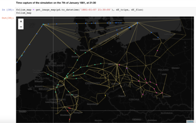
In order to obtain a dynamic visualization, the algorithm creates a random uniform distribution of the number of trains necessay to transport the amount of coal from one city to the next one over the whole year and for each transport line. This results in a fictitious train schedule that extends over a year and whose frequency and routes are realistic and plausible. This simulation is performed at a 5-minute frequency precision and produces a total of 334939 fictitious routes, spread over one whole year. The amount of coal which is transported in each train is estimated based on secondary literature research on American freight transport because it was unavailable on German freight transport: The American Railroad Journal of Aug 1, 1842 admires a train, carrying a 200 tons freight that was drawn from Albany to Boston; while in 1903, an average American freight train can carry a load of about 391 tons. An estimation was made, only as an approximation necessary to give us the correct order of magnitude: since the German rail network was considered well developed by the American standards in the second half of the 19th century, we took the arbitrary number of 330 tons by freight train as an average load.

The visual representation of this simulation is made in the form of a video. In order to create the video representing the coal flux, the html frames are first screenshotted automatically and transformed into png images. The png images are modified in order to add the date and hour in the simulation, using PIL library. In a second time, these images are assembled into a video using imageio library, in order to obtain a dynamic visualization. The video shows the trains in moving dots of different colours, corresponding to the colour code adopted for the map to represent the different coal production locations. The ships that transport coal along the seaways are represented as small moving triangles.

The whole algorithm was coded using Python 3. The interactive maps are in html format and can therefore be easily integrated into any website. Finally, we have created a website allowing the user to interact with the virtually recreated map.

• 

  Production centers

• 

  Production centers, by coal type

• 

  Consumption centers

• 

  Import-export by city

• 

  Transit nodes

• 

  Shipments arrivals

• 

  Shipments departures

• 

  Routes network

• 

  Land routes network

• 

  Naval routes network

Quality assessment

• 

  Quality assessment of production/consumption data

• 

  Quality assessment of transport routes data

• 

  Example of uncertainty : the 7 can sometimes be confounded with the 1

• 

  Example of uncertainty : the direction of the flux with weight 65 is unsure

• 

  Example of uncertainty : surimposed information

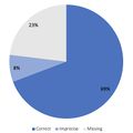
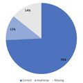
In order to operate a quality assessment of our work, we have decided to randomly test about 10% of our data. For that, we have exchanged our roles in the data entry process. One of us has arbitrarily selected a number of cities on the real historical map representing 10% of the total number of cities on our virtual map in order to see whether or not the city was present and correctly located on the virtual one as well as informed by correct quantity of production and consumption. In the same manner, one of us has arbitrarily selected a number of fluxes on the real historical map representing 10% of the total number of fluxes present on our virtual map to see whether or not the flux was present and correctly located, and whether its quantity and type were correct on the virtual one.

For each test, both the cities and the fluxes, we have categorized our results as either correct, imprecise or missing. By switching roles during that quality assessment process relative to our roles in the data entry process, we have tested the effect of the arbitrariness of selecting the visually most important cities and fluxes from the map in order to de-clutter it. One can notice from the charts above that our uncertainty level is high and can be considered a result of both the imprecision of manual data entry and the slightly random nature of an arbitrary process of selections based on the subjective criteria of visual prominence. Missing data can be caused by different selection choices.

Besides, the errors reported are partly explained by the high complexity of the map and must be put into perspective with this high density of information. Moreover, some journeys between two cities may contain many different coal flows and it is sufficient for one of them to be imprecise for us to consider in our analysis that the data for this flux is imprecise, which is a rather strict criteria. In addition, the colors of the map are sometimes difficult to distinguish, perhaps because of the state of the colors on the original map or the brightness during scanning. This is particularly the case for coal flows represented in brown or beige, which are sometimes difficult to differentiate. Finally, it should be noted that the concentration of information sometimes impacts the readability of the map itself. Some figures may, depending on the interpretation, be attributed to different points on the route and this interpretative variable necessarily impacts the results of our verification, even if it does not inherently affect the quality of the data extracted. To summarize, these data must be clearly interpreted as coming from a partly subjective interpretation and simplification, and therefore subject to a certain uncertainty, but not inherently false.

As our work is based on two different data files, it is important to check that these two files are perfectly coordinated and that each information in the first file can be correctly linked to the entries in the second file and reciprocally. This verification is carried out directly within the program. Thus, we can confirm that 100% of the entries in the first file (.csv routes) find the information related to the arrival and departure cities of the second file (.csv cities). Since the map is interactive, the coordinates of the cities can be visually verified. We have carried out this verification and can also confirm that the contact details are accurate in 100% of cases.

Motivation and description of the website

• 

  Home screen of the website

• 

  Introduction at the bottom of the home page

• 

  Do-it-yourself page

• 

  Naval routes visualization page

• 

  Transport hubs visualization page

• 

  The settings.py file allows the user to adapt the code easily to visualize his own data

Coal is the most important ressource of the industrial nations of the 19th century. Indeed, coal supply was essential to the nation's survival and prosperity at the time. The map we were working on represented the discontinuous flow that irrigated the German Empire, as blood could irrigate a human body. The accessibility of this information is an important historical fact because the Empire's coal supply during this key period built Germany as it exists today. The urban planning and social tissue of many actual cities has been shaped by the coal economy.

More generally, the development of tools enabling the representation of networks and flows of goods is of particular interest to digital humanities. Networks are everywhere: in economics, social sciences, art history. They allow complex phenomena and multiple interactions to be transposed. The exploration of new ways of presenting networks in interactive form also provides a better understanding of abstract concepts and causal relationships between different events.

Our algorithm was designed to allow to separately study the supply and demand of important cities, the trade routes as well as the trade hubs. It will also be possible to view separately the cities which have the main deficits or surplus in production over consumption. It creates the possibly of interacting with a map that was previously static.

To enhance reuse opportunities, we have also created a guideline page on the website for anyone to be able to work with this algorithm in order to analyse any generic dataset of another year on Germany's coal consumption and transport or even completely different flux of goods. The algorithm is conceived in order to be easily reusable by anyone. The user do not have to dig into the code, the settings necessary to fit the model to any project which aims to represent a transport network are grouped in a single settings.py python folder (see thumbnail).

Ultimately, the website, by associating the interactive representation of the data with the historical insights provided by the secondary literature, is drawing the visitor into a very concrete and visual characteristic of Germany's development ten years into its creation as a nation-state.

Project plan and milestones

Project plan

Our goal in this project is to manually extract and to interactively visualize the data on coal production, consumption and transport in 1881 Germany based on a contemporaneous map.

In order to do that, we will first study the map's representation of coal's supply and demand of the German Empire and we will arbitrarily select cities based on their relative importance either as suppliers, consumers or transport hubs. We will then take physical measurements of the map's visual representations and convert those measurements into a numerical dataset based on the map's legend and scale.

Subsequently, we will code an algorithm to treat that dataset and convert it into a dynamic visualization of coal transport flows according to the different mining basins, consumption centers, and transport routes. We will then create a website allowing the user to study separately the supply and demand of important cities, the trade routes as well as the trade hubs. It will also be possible to view separately the cities which have the main deficits or surplus in production over consumption. We would also like to create a guideline page on the website for anyone to be able to reuse the algorithm in order to analyse any generic dataset of another year on Germany's coal consumption and transport or even completely different flux of goods.

Ultimately, we will use that interactive representation of the data in order to try to draw historical insights into Germany's development ten years into its creation as a nation-state. By considering that representation through the prism of secondary literature, we hope to comparatively ascertain the way in which the macroeconomic aspects of German unification preceded its the political unification.

First steps

• Definition of data format
• Bibliography and Research on historical context
• Definition of extraction methodology on
• Extraction done at 40%
• Code the interactive maps of production and consumption centers
• Code the static trade routes map
• Code the dynamic trade routes representation
• Automatisation of the conversion of html maps to png images

Milestone 0 (9.11)

• Complete project plan and milestones on the wiki (>300 words)
• Debriefing on the project progress
• Preparation of midterm presentation

Milestone 1 (14.11)

• Create first version of the website to present maps
• Midterm presentation
• Discuss insight

Milestone 2 (18.11)

• Extraction done at 65%
• Motivation and description of the services (> 200 words)
• Update website main page with motivation and description of the services
• Add the color dimension to the interactive visualisation of production centers (mining basins)

Milestone 3 (25.11)

• Extraction done at 100%
• Run algorithm of interactive maps (consumption, production, transport hubs, etc.) on all the data set
• Update the website with full interactive maps
• Document the wiki with the detailed description of the extraction methods (> 500 words)
• Document the wiki with quantitative analysis of the performances of extraction (> 300 words)
• Create a page with detailed description of the extraction methods on the website and quantitative analysis of the performances of extraction

Milestone 4 (2.12)

• Add the color dimension the the dynamic simulation of the data set (mining basins)
• Test dynamic simulation with the full data set
• Check dynamic simulation for bugs
• Automatisation of the conversion of png frames to gif animation
• Document the wiki with historical introduction to the map (> 200 words)
• Create a page with historical introduction to the map on the website

Milestone 5 (9.12)

• Make dynamic simulation displayable on the website
• Enrich the wiki and the website with historical analysis of the subject
• Add guideline page on the website for anyone to be able to reuse the algorithm in order to analyse any generic dataset

Milestone 6 (14.12)

• Deliver Github repository
• Prepare final project presentation

Milestone 7 (19.12)

• Final project presentation

Further possible upgrades

• Finding a way to make the website generic: if another data set was available (either a different time or a different commodity), could it be processed by our algorithm and be represented graphically in an easy way.
• Compare the supply of the time with an optimized computerized supply.
• Further analyze coal consumption data by cities in relation to the main industries of the time.
• Observe the correlation of coal production and consumption at the time with the level of subsequent economic development of cities, in an attempt to quantify the economic impact of this strategic resource.
• Highlighting the possible parallels between the role of coal in the German unification and the European unification (European Coal and Steel Community).

Links

• Link to the project website
• Link to the GitHub repository containing the project code
• Link to the map on Gallica
• Link to the Jupyter notebook viewer which contains all the interactive maps

References

- ↑ 1.0 1.1 1.2 Toni Pierenkemper, Richard H. Tilly, The German Economy During the Nineteenth Century pp. 59-70.
- ↑ 2.0 2.1 Arnold H. Price, The Evolution of the Zollverein: A Study of the Ideals and Institutions Leading to German Economic Unification between 1815 and 1833 (Ann Arbor: University of Michigan Press, 1949) pp. 9–10.
- ↑ David T. Murphy, "Prussian aims for the Zollverein, 1828-1833", Historian, Winter 1991, Vol. 53#2, pp. 285-302.
- ↑ David J. S. King, "The Ideology Behind a Business Activity: The Case of the Nuremberg-Fürth Railway", Business and Economic History, 1991, Vol. 20, pp. 162-170.
- ↑ The Brooklyn Historic Railway Association, Brooklyn, NY. <http://www.brooklynrail.net/science_of_railway_locomotion.html>
- ↑ Tom Morrison, The American Steam Locomotive in the Twentieth Century, McFarland, 2018, p. 37.