Influencers of the past

Abstract

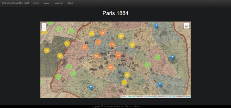
The goal of this project is to show who were the notable people in Paris in 1884 and 1908 and where they lived. Our expected output is a webpage showing both maps from 1884 and 1908, with clusters indicating the number of inhabitants. The more you zoom, the more details you can see. You can click on a point to have more information about someone (i.e. his/her name). We will provide an analysis of the results.

Here is the initial sketch of our project: Sketch of Influencers of the past and you can find the final website at the following link: Project website.

Preview of our website

Planning

Task	Status	Deadline
Extract the data	Done	(:
Clean the data	Done	(:
Get coordinates of the addresses	Done	22.11.19
Georeference old maps	Done	22.11.19
Display people on maps	Done	29.11.19
Web interface and analysis	Done	06.12.19

Historical sources

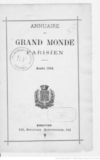
In this project we are dealing with two main sources: the Annuaire du grand monde parisien of 1884 and the Paris-mondain: annuaire du grand monde parisien et de la colonie étrangère of 1908. These annuaires comprehend a list of people considered famous and influential at the time, listing for each of them their names and addresses. As stated in the preface by the author of the 1884 annuaire, Pol Hanin, the goal of such a book was to honor the high society of Paris and create a truly useful list of famous people.

For the visualization, we have used two old maps of Paris. For the year 1884, we have the Nouveau plan complet illustré de la ville de Paris en 1884 by Alexandre Aimé Vuillemin and Charles Dyonnet. For the year 1908, we have the Plan de Paris, Mars 1908 et du chemin de fer métropolitain, distinguant les lignes déclarées d'utilité publique; les lignes concédées à titre éventuel et la concession de la Cie Nord-Sud by L. Wuhrer. Both maps are stored at the Bibliothèque nationale de France, in the departement Cartes et plans. Note that the second map also presents the subway network of Paris at the time, of which the first line was opened on July 19th of 1900 for the Olympics Games of that year.

Annuaire du grand monde parisien (1884)	Paris-mondain: annuaire du grand monde parisien et de la colonie étrangère (1908)

Main steps

Extracting the data from the directories

Our first step is to extract all the names and addresses from the two directories. To do so, we use Transkribus to get the OCR and then start to parse the information.

Cleaning the data

This is the principal step in our project. The data the OCR gives us is quite messy, there are a lot of errors and we definitely need to correct them to hope obtaining the coordinates of our addresses. We also need to harmonize our results. For instance, we want to consider in the same way 'r.' and 'rue' (the French name for 'street') or 'bd' and 'boulevard'. Having all our addresses in a standardized form is also helpful to easily retrieve the corresponding coordinates. The principal challenge of this step, is that we have two different OCRs for the two years (1884 and 1908). We thus had to implement two specific parsers.

The code for the parsers can be found here: 1884 parser and 1908 parser.

Cleaning the 1884 annuaire

The format for the 1884 OCR was xlsx. Since the results were given in small tables of a dozen of elements each but with a different number of columns each time (2, 3, 4 or 5), first we had to combine all our results in one single DataFrame with two columns: Addresses and Names. Then we have proceeded with the cleaning of each column.

Addresses

For the addresses, we have based our cleaning on the work done by Peter Norvig. The idea of this spelling corrector is to manually correct some addresses to learn the correct spellings and store the corrected words. Once this is done, the actual corrections are performed: word by word, we find all the words at edit distances 1 and 2 that are in the list of corrected words and replace it with the most probable correction. This is well-suited for correcting addresses since we have many occurrences of the same words (such as "rue" or "bd"). Once this is done, with a last few corrections on specific cases (simply using the replace() method for strings in Python), we can get the coordinates of each address.

Names

We also need to clean the names but this is much harder since there cannot be a list of "corrected names". What we can do, however, is correct the titles. Indeed, in the 1884 annuaire, many people's names come with their title (such as "Cte" for "Comte"). We therefore use a simple dict to map the abbreviations (and their different occurrences, due to OCR errors) to the full title. We also correct some specific cases such as "cl'" instead of "d'". The last thing we have done is splitting the spouses as in many cases they were listed together. This has increased the number of people by approximately 500 people. In the end, we have decided to keep the households (not split) in the visualization but these results could still be used for further analysis.

Cleaning the 1908 annuaire

The format for the 1908 OCR was txt. By looking at the raw data from the OCR, we saw that most of the people were separated by a '\n', or were at least on different lines. Also, each new entry starts with the name of the person in uppercase and every information about him/her is separated by a comma.

We use these criteria to separate the people and put them into an array. Concretely to detect a new person, we check:

1) If the line is a '\n'

2) If the line starts with a family name i.e if at least 60% of the first word of the line is in uppercase. This threshold allows us to tolerate small OCR errors

We also split every people in our array by comma. Then, each entry of our array is an array which contains the name of the person as a first element. We retrieve his/her address with helpers methods.

Addresses

To find the address of a person, we iterate over the entry and look for a digit (or a digit followed by "bis"). This is because we noticed that most of the addresses start with the street number of the address. Once the digit is found, we concatenate all the following elements of the array until we hit a '('. This is because every address ends with "('arrondissement' number)" and we don't need it.

Names

Once we have the addresses, we need to clean the names which have a lot of parasitic characters. We then also wrote a few helpers methods.

Example:

We want to obtain "Aurélie Capece ZURLO" from "ZURLO (P"*«“ Aurélie Capece)"

To retrieve the first name, we have the following criteria:

• Starts with an uppercase character
• Is mostly composed of alphanumeric characters (we tolerate OCR mistakes)
• Apart from the first character, the first name is mostly lowercase (we also tolerate OCR mistakes)

To retrieve the last name, we have similar criteria as explained in the parsing phase (i.e. more that 60% of uppercase characters). We also replace '1' by 'I' and '0' by 'O' as we noticed it was a frequent OCR mistake. In the end, we keep only the alphanumeric characters.

If we detect the word "née" ("born" in french), it means that the entry contains as well the name of the spouse of the person. We then retrieve the last name of the spouse (the name following "née"), and write "HUSBAND-NAME et Mme née WIFE-NAME".

This gives us a pretty clean DataFrame with names and addresses.

Finding the geolocation of the addresses

To be able to show the addresses on the map, we need to find their geolocation (latitude/longitude coordinates). For this step, we have proceeded in two steps. First we have used the list of addresses of Paris created by the DHLab. This database provides a list of old Paris addresses with the start and ending date (if known) and the coordinates (latitude and longitude, directly in the format EPSG:3857 handled by Leaflet). The difficulty was to ensure the matching of the addresses between our lists and the database. To do so, we have designed a "normalized" way of representing the addresses (removing all the accents, the punctuation, setting all the letters to lowercase and putting the number at the end).

As a lot of addresses were still missing, we used the GeoPy API to complete our database.

We wrote a script that iterate over the remaining addresses and send a request to GeoPy to get the corresponding coordinates. However, that works for approximately 1000 requests before being blocked for "too many requests" for 24 hours. Then we had to run our script multiple times, to get all addresses.

Georeference old maps of Paris

Once we have the coordinates of our addresses we need to georeference old maps of Paris. To do so we first used Georeferencer to get our old maps in the format TIFF. Through the localization of homologous points between the old map and the present map, this tool allows to project coordinates on the old map.

However, Georeferencer did not seem to work anymore. Indeed, it was neither possible to get working URLs for our maps nor the TIFF versions of them. QGIS was finally used to georeference the maps and get the TIFF models. We then used gdal2tiles to generate the tiles of the maps, which can be used with the library Leaflet to visualize our results.

Visualize results

Once we have all our elements we can start visualizing our results. At first we tried to continue using Python with the Python module Folium (implementing Leaflet). However the results were not great: it would take a long time to load and we would not have much control on how to visualize the people. This is why we have decided to switch to Javascript, making it also much simpler to embed the maps in our website. Then we had to decide how to display the famous people on the map. The naive way would be to simply put all our addresses on the map as markers but due to the large number of addresses we have (a few thousands) this would result in a overcrowded map. Our first idea is therefore to cluster our addresses when they are near each other. This will allow, at low level zoom, to visualize 'influential' neighborhoods for instance. Then, when one starts to zoom more on the map, he will eventually reach a level where each person is shown as a dot. In this last case, when one clicks on the dot, a pop-up with additional information on the person (such as the name) will show up. To do so we use the Leaflet plugin MarkerCluster. This is a first step to show how "clustered" the famous people are but we want to implement other visualization to better show it. The first one use the Leaflet plugin Heat, a simple heatmap plugin, to represent the density of famous people. The second one adds to the map the arrondissements of Paris, coloring them given the number of famous people within. Finally, the same thing is done with the quarters of Paris. Notice that both the arrondissements and the quarters date from 1860 and have not changed much up to the present day, meaning that finding the fanciest quarters is meaningful (even without knowing the precise history of Paris).

Quality assessment

In this section, we assess the quality of our processes. First we evaluate the quality of our parsing of the OCR output, comparing the number of entries in the annuaire and the number of addresses we have to clean. Note that for the 1908 list, the OCR has given us a text file and therefore this evaluation will combine both the quality of the OCR and the quality of our parsing methods to extract each pair name/address. For the 1884 list, the OCR directly gives us a table of names and addresses, thus this evaluation assesses the quality of the OCR, over which we have no control. To estimate the number of entries in the actual annuaire, we have counted them manually on a few pages to get the mean number of people per page (a very constant number due to the clear structure of the annuaires) and multiplied it by the number of pages. We get the following results:

Year	Entries per page	Number of pages	Total number of entries	Output of the OCR	After removing missing values	Quality assessment [%]
1884	35	182	~6400	5709	5590	87
1908	40	310	~12400	11045	9684	78

Then we need to evaluate the quality of our cleaning on the addresses and how many coordinates we managed to get. Those two steps are evaluated together as the quality of our cleaning directly reflect on the number of coordinates we get. Here are the results:

Year	Entries pre-cleaning	Entries with coordinates	Quality assessment [%]
1884	5590	3572	64
1908	9684	5295	63

Example of a hard-to-read address in the 1908 annuaire

Overall we have managed to get the coordinates of 56% of the people in the 1884 annuaire and 43% of the people in the 1908 annuaire. This numbers seem to be quite low but it is important to stress out that, especially for the 1908 entries, the OCR output was of poor quality. This was to be expected as the 1908 annuaire itself has less structure than the 1884 one and the quality of the images on Gallica is poorer. In some cases, even for a human it would be hard to read the exact information, as in the following example.

Analysis of results

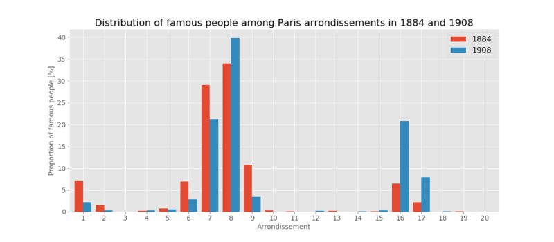
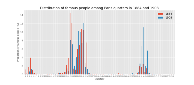
We have counted the number of people within each arrondissement and each quarter for both years and normalized the results by the total number of famous people of that particular year. We present the results in two bar plot.

As it was already observed on the maps, in 1884 the famous people seem to be clustered in a few arrondissements, namely the 7th and the 8th. This is not surprising, as still today those are the richest and fanciest arrondissements of Paris, with the Champs-Elysées or Place de la Concorde. What is however more interesting is the shift that can be observed in 1908. It seems that the famous people left the 1st, the 6th, the 7th and the 9th arrondissements moving towards the 16th and the 17th, situated outside the center of Paris. Notably, the 16th arrondissement, Passy, had been annexed to Paris only in 1860, due to Paris expansion with the June 16th 1859 law. With the opening of the first subway lines in 1900, moving around in the city was much easier and this might have encouraged famous people to move towards the border of the city.

With this second graph we can observe more in detail the repartition of famous people in Paris and the shift between the two periods. Using the 1908 map, we can notice that the quarters populated with the most famous people are the one when the already functioning lines are passing. Particularly central seems to be Place de l'Etoile, where multiple important streets and subway lines cross, at the corner between the 29th, the 30th, the 64th and the 65th (four among the more "famously" populated quarters of Paris).

Further analysis could focus on specific subway stations but more data would be needed in order to obtain significant results.

Links

• Project website
• Github repository hosting the website
• Github repository for cleaning

References

- ↑ Preface of the Annuaire du grand monde parisien, 1884
- ↑ Gustave Fulgence, « Le plan de métro de Paris revisité », Confins (Online), 30; posted on February 24th 2017, seen on December 8th 2019; DOI : 10.4000/confins.11869
- ↑ Transkribus
- ↑ How to Write a Spelling Corrector, by Peter Norvig, posted on Feb 2007 to August 2016
- ↑ Leaflet
- ↑ GeoPy Contributors, "GeoPy Documentation", posted on 26/05/2019
- ↑ Georeferencer
- ↑ QGIS
- ↑ gdal2tiles plugin
- ↑ "Folium documentation"
- ↑ Leaflet.markercluster
- ↑ Leaflet.heat
- ↑ "Geocoordinates of Paris arrondissements
- ↑ "Geocoordinates of Paris quarters
- ↑ "Historical quarters of Paris
- ↑ Brief history of the Paris metro, by france.fr