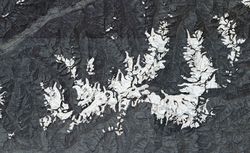
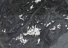
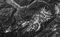
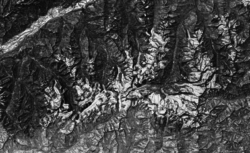
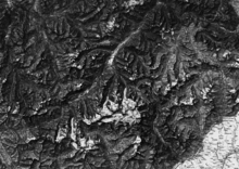
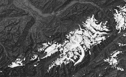
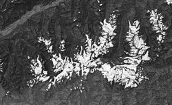
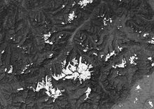
Detection of glacier change using dhSegment from the Siegfried map from 1874
Introduction and Motivation
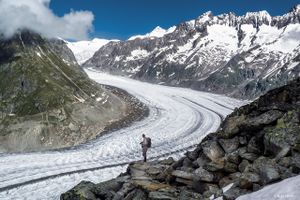
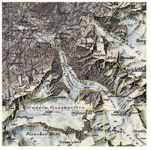
Swiss glaciers are a prominent feature of the Swiss landscape and are a source of pride for the country. They are formed when snow accumulates over many years and compresses into ice. As the ice becomes denser and heavier, it begins to flow downhill under the force of gravity. Swiss glaciers are found in the Alps, which run through the central part of the country. There are approximately 1,800 glaciers in Switzerland, which cover about 1,200 square kilometers of the country's surface. Swiss glaciers are an important source of water for the country, as they melt in the summer months and provide a steady supply of water to rivers and streams. Glaciers are important indicators of climate change and are sensitive to temperature fluctuations. In recent years, Swiss glaciers have been retreating due to rising temperatures, which has led to concerns about the impact on the local environment and economy.
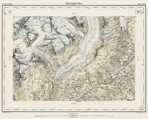
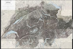
The Siegfried Map, also known as the Topographic Atlas of Switzerland, is an official series of maps of Switzerland. It was first published by the Federal Topographic Bureau under Hermann Siegfried in 1870 and continued to be produced until 1926. The maps in this series were drawn by a variety of lithographers, including Walter Hauenstein, Georg Christian von Hoven, and Rudolf Leuzinger. The Siegfried Map is considered an important resource for those interested in the geography and topography of Switzerland, as it provides detailed and accurate representations of the country's landscape and features. It is sometimes referred to as the "Siegfried Atlas" or the "Siegfriedkarte," although it is technically a map series rather than an atlas.
In our project, we want to combine the above two concepts. That means unearthing hidden glacier information behind Siegfried Maps from different years. On the one hand, we can train a model based on the map to predict the glacier area from the map. On the other hand, we want to discover the changes in the glacier area through the predicted results in different years.
Methodology
Build Dataset
Data collection
map.geo is a website operated by the Swiss Federal Office of Topography (Swisstopo), the national mapping agency of Switzerland. The website provides a range of online mapping services and tools for users to access and explore geographical data for Switzerland. The website provides a range of map services that allow users to access and use the geospatial data and maps provided by Swisstopo in their own applications and websites. These services include web map tiles, feature data, and geocoding services. Overall, map.geo.admin.ch is a valuable resource for anyone interested in exploring and using geospatial data and maps for Switzerland. The whole map is divided into numerous small square patches and each piece is corresponding with a formatted URL including columns and row information. So our first step is to obtain cropped images and stitch them into a complete map image in a specific order. For web scraping, we primarily use requests package in python to resolve the response and store the data locally.
Data annotation
After obtaining the whole map images, we first choose a proper size of a single training picture and crop the whole map into pieces of that size. We looked at a combination of two factors in choosing single picture size.
- Detail level: The size of the training images should be large enough to capture the level of detail that is relevant to the task. For example, if the task requires the model to identify small objects or features, you may need to use larger training images to provide enough context for the model to accurately identify those features.
- Memory constraints: Larger training images require more memory to process and store, so you may need to use smaller training images if you have limited hardware resources.
And finally after some experiments, we made the decision to crop it into 1024*1024 size with 256 pixel overlap for each adjacent image. We then generate the annotated glacier label on the map to carry out subsequent model training. Since the labeled data cannot be obtained directly, we tried a variety of methods for data labeling.
Automatically match using Georeference
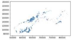
The Swiss Glacier Inventory 1931 is a comprehensive record of glaciers in Switzerland that was created by the Swiss Federal Office of Topography (Swisstopo) in the 1930s. The inventory was based on field surveys and aerial photographs taken in the late 1920s and early 1930s, and it includes detailed information on the size, shape, and location of more than 3,000 glaciers in Switzerland. It provides areas and outlines of all glaciers in Switzerland referring to the year 1931. The data are based on terrestrial imagery and are delivered as a shapefile, which describes the shape of the glacier and give its position in the CH1903 geographical coordinate system. So the task is that matching every pixels with CH1903 geographical coordinate now.
The data are based on terrestrial imagery and are delivered as a shapefile, which describes the shape of the glacier and give its position in the CH1903 geographical coordinate system. So the task is that matching every pixels with CH1903 geographical coordinate now. We tried two methods to match the pixels:
- Manual calculation
- QGIS tools.
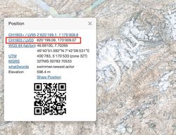
Manual calculation means that if we know the geographical coordinates of the four corners, we can calculate the geographical coordinates of each pixel by converting the relationship between pixels and geographical coordinate units.
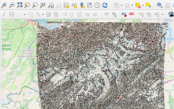
Using QGIS tool means georeferencing the images by QGIS, a geographic information system application. Reference points between the glacier image and a CH1903 reference map are identified manually and from which, we will obtain a quadratic or cubic polynomial as pixel point and geographical coordinate conversion formula.
After we have geographic coordinates of each pixel, for each pixel (x,y) in the image, transform it to geographic coordinates (n,m) using georeferencing. Then, check whether the pixel is within the boundaries of the glaciers. If it is within the boundaries, label the pixel as "glacier." If it is not within the boundaries, label the pixel as "non-glacier." Repeat this process for every pixel in the image to create a map of the glaciers, Both methods will generate the label image that is the same size as the original image.
Manually annotation using VGG Image annotator
VGG Image Annotator (VIA) is a free, open-source, web-based tool for annotating images and videos. In this method, we don’t need geographic coordinate information. We simply label and annotate glacier areas by hand using VIA. This tool allows you to easily draw bounding boxes around objects in an image, as well as import and export annotations in a variety of formats. In our project the export format is JSON and we convert them to images based on the original image size.
During labeling with VIA, we strictly distinguished the boundaries of the glacier. For example, in the case of mountain ridges, glaciers form when snow and ice accumulate over time, and the weight of the accumulated snow and ice causes it to compress and turn into ice. The ice in a glacier flows slowly downslope due to gravity, and as it moves, it erodes and shapes the landscape. So sometimes a glacier is located at a lower elevation instead of the ridge area. Although the area size is minor compared to adjacent glacier, but we still label it out rigorously.
Method Comparation and Selection
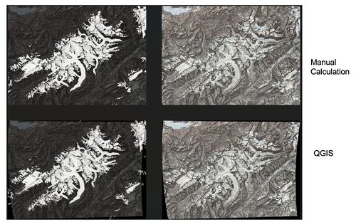
After exploring the two options mentioned above, for the first method, we encountered issues with accuracy due to discrepancies between our map and the reference map. These differences, such as the deviation between the white glacier on the original map and the annotation, were noticeable to the naked eye and would have negatively impacted the training of our model. In the same situation, we can see that the label using VIA is more consistent with the original data. In order to achieve a more accurate and effective model, we decided to use the manual VIA method. However, this manual process can be time-consuming and may not be feasible for large datasets. Despite these challenges, we believe that the improved accuracy of the model is worth the additional effort.
Build Model and Prediction Pipeline
Model introduction
MMSegmentation is a highly regarded open-source library for image segmentation in Python that is built on the PyTorch deep learning framework. It offers a wide range of tools and algorithms for training and evaluating image segmentation models, making it a popular choice among researchers and developers working on image segmentation projects. The library is designed to be user-friendly and flexible, allowing it to be utilized in a variety of applications. MMSegmentation has seen widespread adoption in fields such as computer vision, medical imaging, and autonomous vehicles, to name a few. Its versatility and ease of use make it a valuable resource for anyone looking to tackle image segmentation tasks.
Based on MMSegmentation, we selected three advanced model: ICNet, FastSCNN and OcrNet.
ICNet
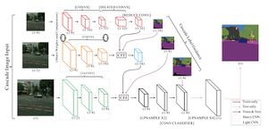
Interleaved Convolutional Networks (ICNet) is a real-time semantic segmentation model that is able to handle high-resolution images effectively. It is a multi-scale, multi-path network that utilizes a combination of convolutional neural networks (CNNs) and a cascaded structure to achieve fast and accurate segmentation results. ICNet has three branches: a high-resolution branch, a mid-resolution branch, and a low-resolution branch, each of which processes the input image at a different resolution and combines the outputs to generate the final segmentation. One notable feature of ICNet is its use of a pyramid pooling module, which enables the model to adapt to a wide range of scales and shapes within the input image. This allows it to accurately segment small objects, as well as objects that are occluded or partially visible.
FastSCNN
Fast Segmentation Convolutional Neural Network (Fast-SCNN) is a real-time semantic segmentation model that is designed to provide fast and accurate segmentation of images and video frames, with a particular focus on real-time performance. It is a lightweight and efficient model that can be easily implemented on resource-constrained devices, such as mobile phones and embedded systems. Fast-SCNN uses depthwise separable convolutions and a global context module to efficiently extract features from the input image, and a multi-scale input representation to capture context at different scales. Additionally, Fast-SCNN employs a hybrid training strategy that combines supervised and self-supervised learning, allowing the model to learn from labeled data as well as data generated by applying transformations to the input images. Overall, Fast-SCNN is a versatile and effective model for real-time semantic segmentation tasks.
OcrNet
Object-contextual representations(Ocr) are a type of representation used in the field of semantic segmentation, a task in computer vision that involves labeling each pixel in an image with a semantic class. These representations encode both object-level information (i.e. information about specific objects in the image) and contextual information (i.e. information about the relationships between objects and the larger scene). There are several approaches to creating object-contextual representations, including using a combination of convolutional neural networks (CNNs) and recurrent neural networks (RNNs) or using graph convolutional networks. Object-contextual representations are useful for tasks such as scene understanding and image captioning, as they help capture the relationships between objects and their context, which is essential for understanding the meaning and significance of the objects in the image.
Greyscale case
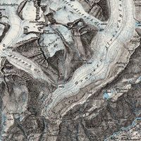
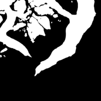
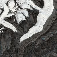
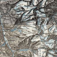
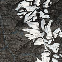
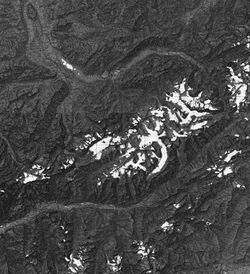
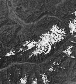
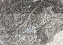
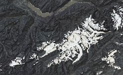
Our target years for prediction are 1884-1935, but maps prior to 1905 are in black and white. Since our training dataset are colorful maps from 1931, the prediction results on black and white images were not satisfactory due to a lack of color information. To improve the model's performance on these images, we converted the 1931 training images from RGB to grayscale and trained a new OcrNet model (distinguished as OcrNet-RGB and OcrNet-Grayscale in the table below). As shown in the figure below (from left to right: original map in 1890, prediction based on OcrNet-RGB in 1890, prediction based on OcrNet-Grayscale in 1890), it demonstrates that this approach is effective in improving the model's performance and discover more glaciers on black and white images. We will discuss these results in more detail in the next section.
Training settings
We trained all three models using a pre-trained strategy. This means that we started with a pre-trained model, such as the one provided by MMSegmentation, and fine-tuned it for our specific task of glacier segmentation. Using a pre-trained model allows us to leverage the knowledge that the model has already learned from a large dataset, which can help to improve its performance on the new task. Below, we provide the training settings and configuration files that we used for MMSegmentation.
| Data split | Model architecture (Backbone Network) | Optimization (learning rate, momentum, weight decay, and batch size) | Training details (epochs, frequency of validation) | Hardware/Software | |
|---|---|---|---|---|---|
| OcrNet-RGB | 195 pairs for training, 39 pairs for validation | HRNetV2p-W18-Small | SGD(0.01, 0.9, 0.0005, 2) | 2000 iters, per 200 iters a validation | Tesla V100 32GB/pytorch 1.13.0+cu116/mmsegmentation 0.29.1 |
| OcrNet-GreyScale | 195 pairs for training, 39 pairs for validation (all images are grey scale images) | HRNetV2p-W18-Small | SGD(0.01, 0.9, 0.0005, 2) | 2000 iters, per 200 iters a validation | Tesla V100 32GB/pytorch 1.13.0+cu116/mmsegmentation 0.29.1 |
| ICNet | 195 pairs for training, 39 pairs for validation | ResNet-101-D8 | SGD(0.01, 0.9, 0.0005, 4) | 2000 iters, per 200 iters a validation | Tesla V100 32GB/pytorch 1.13.0+cu116/mmsegmentation 0.29.1 |
| Fast-SCNN | 195 pairs for training, 39 pairs for validation | FastSCNN | SGD(0.12, 0.9, 4e-05, 4) | 2000 iters, per 200 iters a validation | Tesla V100 32GB/pytorch 1.13.0+cu116/mmsegmentation 0.29.1 |
Prediction
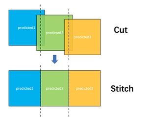
We have selected three glacier concentrations in Switzerland and projected and analysed them over a 60-year horizon. Our steps are to first stitch together a large image of the selected region using the meta images on the website, then cut it into small images of 1024*1024 with a 256 overlap between adjacent pieces as our to-be-predict data. Depending on the type of image to be predicted (RGB or grayscale) we feed these pieces into our model to obtain the glacier prediction results. Then stitching them together to get a whole view of the area, because there is an overlap between each pair of two adjacent images, our strategy is taking half from each of the overlapping parts which means keeping the 128 pixels closest to the image itself. The reason for doing this is that deep learning segmentation models tend to produce poor results when predicting area near image edges, and using an overlapping prediction strategy will improve the accuracy of our predictions.
Result and Quality Assessment
Assesment & Model Selection
To evaluate the performance of our model, we will introduce three concepts: PA(Pixel Accuracy), IoU(Interaction over Union), MIoU(Mean Interaction over Union).
PA(Pixel Accuracy) in our model reflects the proportion of correctly classified pixels in the image compared to the total number of pixels. One advantage of this metric is its simplicity. However, it has a disadvantage when evaluating the image segmentation performance of small targets. If a large area of the image consists of the background and the target is small, the accuracy score may be high even if the entire image is predicted as the background, making it an unreliable metric for small target evaluation.
There are a total of k+1 classes in the image. Pii represents the number of pixels that are correctly classified as class i (number of pixels correctly classified), and Pij represents the number of pixels that are incorrectly classified as class j for all i and j (All pixel count).
IoU stands for "intersection over union," and is a measure of the overlap between the predicted values and the true values in a classification task. IoU is not only used in semantic segmentation, but also one of the commonly used indicators in object detection.
To calculate the IoU for class i, the numerator is the number of pixels Pii that are correctly classified as class i. The denominator is the sum of the number of pixels with a label of class i and the number of pixels classified as class i, minus the number of pixels correctly classified as class i.
MIoU stands for "mean intersection over union," and is the average IOU across all classes in a classification task. The mean IoU is then computed by taking the average of the IoUs for each class."
We ultimately chose the IoU for the "glacier" class as the main evaluation metric for our model because our model can classify the pixels in the input image into two classes: background and glacier. Our task is to find the area of the glacier, so we are more concerned with the accuracy of identifying the glacier. Therefore, we choose the IoU for the glacier class as the metric and regard OcrNet as our primary model since the IoU approaches 87% in our validation. We must also note that although the model is the same as OcrNet, OcrNet-Grey uses grayscale images for training and is missing RGB information, so the prediction results of this model are lower than those of OcrNet-RGB.
| IoU(glacier) | IoU(background) | mIoU | PA(glacier) | PA(background) | mPA | aPA | |
|---|---|---|---|---|---|---|---|
| OcrNet-Grey | 80.04 | 98.37 | 89.21 | 84.59 | 99.56 | 92.07 | 98.47 |
| OcrNet-RGB | 87.71 | 98.13 | 92.92 | 92.75 | 99.17 | 95.96 | 98.35 |
| ICNet | 85.59 | 97.8 | 91.7 | 91.13 | 99.06 | 95.1 | 98.06 |
| Fast-SCNN | 85.11 | 97.71 | 91.41 | 91.37 | 98.93 | 95.15 | 97.97 |
mPA: mean Accuracy, aPA: arithmetic mean Accuracy
Result
We divide the presentation of our results into two parts, in the first part we show the power of our model to predict glacier areas in colour and in grey scale maps. In the second part we use the results from the first part to explore the evolution of Swiss glaciers over a span of nearly 60 years.
Model Prediction
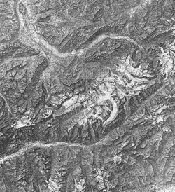
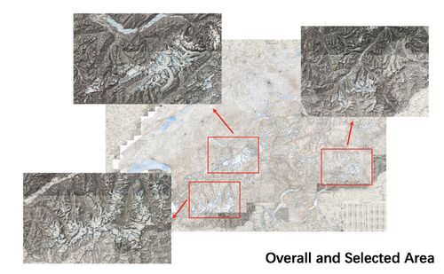
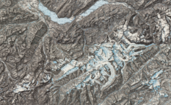
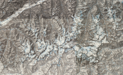
In order to facilitate the development of the subsequent study, we have chosen three glacier-concentrated areas of Switzerland for our study, the locations of the three areas are shown in the figure below. For the three areas we present our predictions using RGB images from 1935 and grey-scale images from 1890 as a sample and all of the results can be viewed in our google drive.
Changes within 60 years
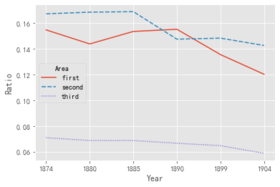
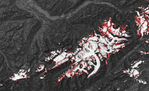
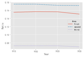
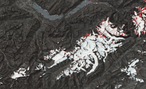
Since the model accuracy of OcrNet-Grey and OcrNet-RGB are different, we believe that direct comparison of the results predicted by these two models to obtain conclusions about glacier changes over time is unreliable, so we divided the entire six decades into two time periods, the first from 1874 to 1904, during which the map data provided by the site are all grey-scale images, and the other from 1915 to 1935, during which the map data provided by the site are RGB images. For each of the years in the period, we calculated the proportion of glacial pixel points out of all pixel points in the area, tabulated and produced a trend graph. Further, to show the glacier changes more clearly, we overlaid the two predicted maps at the beginning and end of each time period and labelled the glaciers that had melted in an alternative color.
For the period of 1874 to 1904, from the table and trending graph below, we observe a decreasing trend in both three areas within the 30 years and the ratio of glacier decrease 22.3%, 14.7% and 17.1% respectively, which is a great loss. The conclusion can also be generated from the loss condition between 1874 and 1904 where we made a deduction of glacier in 1874 and glacier in 1904. The edge of nearly every glacier blocks are melt and shrinked as we annotated in the picture.
| 1874 | 1880 | 1885 | 1890 | 1899 | 1904 | |
|---|---|---|---|---|---|---|
| Area 1 | 15.46 | 14.37 | 15.34 | 15.51 | 13.54 | 12.01 |
| Area 2 | 16.71 | 16.84 | 16.88 | 14.74 | 14.82 | 14.25 |
| Area 3 | 7.08 | 6.86 | 6.86 | 6.65 | 6.46 | 5.87 |
For the period of 1915 to 1935, from the table and trending graph below, we observe a decreasing trend in both three areas within the 30 years and the ratio of glacier decrease 2.9%, 1.9% and 3.6% respectively, which is a great loss. The conclusion can also be generated from the loss condition between 1874 and 1904 where we made a deduction of glacier in 1874 and glacier in 1904. The edge of nearly every glacier blocks are melt and shrinked as we annotated in the picture.
| 1915 | 1920 | 1925 | 1935 | |
|---|---|---|---|---|
| Area 1 | 15.52 | 15.66 | 15.63 | 15.07 |
| Area 2 | 17.51 | 17.51 | 17.22 | 17.17 |
| Area 3 | 7.26 | 7.26 | 7.27 | 7.0 |
Swiss glaciers have undergone significant changes in the period from 1874 to 1935. During this time, many of the country's glaciers retreated significantly due to rising temperatures. This retreat was particularly pronounced in the second half of the 19th century, with many glaciers losing a significant portion of their mass.
The retreat of Swiss glaciers has had a number of consequences, including changes in the availability of water for hydroelectric power generation, increased flood risk in some areas, and loss of habitat for certain plant and animal species. It is important for people to understand and address the causes of glacier retreat in order to mitigate these impacts and protect these important natural resources.
Limitations of the Project
Complex and confused backgrounds
Image segmentation can be challenging when the background is complex and contains objects that are similar in appearance to the objects of interest. In our project, our model relies on RGB information to determine if an area is a glacier, and because the color of a lake is similar to that of a glacier, in some cases our model incorrectly identifies a lake as a glacier.
Overfitting
Image segmentation models may have a tendency to overfit to the training data, leading to poor generalization to new data. Despite the effort we put into annotating the dataset (elaborate annotations took up to five minutes per image), our training data pales in comparison to the huge image data corresponding to the year we are trying to predict, so we still suffer from the inadequacy of the training dataset and the resulting overfitting problem.
Model accuracy
The inability to continuously analyze glacier changes between years due to inconsistencies in the accuracy of the grey-scale and RGB models. Due to the low accuracy of the grey-scale model predictions(IoU 80 vs 87), we can see in the results section that the overall proportion of pre-1910 glacier sections is lower than the proportion of post-1910 glaciers.
Future Work
1. Labeling more data can be a useful way to expand the training set and improve the performance of the model. There are a few different approaches we can take to label more data:
- Manual labeling: we canstill manually label data ourselves. This can be time-consuming but we can ensure the high-quality labels.
- Crowdsourcing: we can use platforms like Amazon Mechanical Turk or Crowdflower to have data labeled by a large group of people. This can be a cost-effective option, but the quality of the labels may vary.
2. The performance of the predicting grey-scale map is not ideal enough, we aim to improve the accuracy to a level that is approximately equal to that of the RGB model. we would explore models based on Transformers or develop ways that depend less on color information or combining their predictions using techniques like bagging or boosting. This can often improve the performance of the final model.
3. Deeper research: What happened during the year range 1874 to 1904? Why do the changes so dramatic in comparation with year range 1915 to 1935? Do the mean temparatures within those years change a lot? We have so many curiosity about the result we have.
Project Plan and Milestones
Project Plan
| Date | Task | Completion |
|---|---|---|
| By Week 3 |
|
✓ |
| By Week 4 |
|
✓ |
| By Week 5 |
|
✓ |
| By Week 6-7 |
|
✓ |
| By Week 8-9 |
|
✓ |
| By Week 10 |
|
✓ |
| By Week 11 |
|
✓ |
| By Week 12-13 |
|
✓ |
| By Week 14 |
|
✓ |
| By Week 15 |
|
✓ |
Milestones
- Different Siegfried Map images extracted from the website (http://geo.admin.ch/).
- Preprocessed (cropped and resized) patches of the raw maps image.
- 234 annotated images (1024 * 1024) of the glacier area and corresponding JSON file.
- Trained segmentation model for the glacier.
- Code and instructions to reproduce the results on GitHub.
Deliverables
Source Code: Github Link
234 manually labeled training dataset: Google Drive Link
11 years of 3 areas detailed result: Google Drive Link
4 trained models and training logs Google Drive Link
Reference
- [1] Maps of Switzerland
- [2] Segmentation Transformer: Object-Contextual Representations for Semantic Segmentation
- [3] ICNet for Real-Time Semantic Segmentation on High-Resolution Images
- [4] Fast-SCNN: Fast Semantic Segmentation Network
- [5] OpenMMLab
