Photorealistic rendering of painting + Venice Underwater

Abstract

The main goal of our project is to automatically transform old paintings and drawings of Venice into a photorealistic representation of the past, thus create photos never taken. In order to achieve this goal, we will utilize style transfer generative adversarial networks to learn what separates a drawing or painting from a photograph and then utilize that model.

After a review of the current literature in the field, we settled on implementing the relatively new contrastive unpaired translation GAN with some key modifications. In particular we plan to build a new auxiliary loss function to enforce geometric continuity between generated and original building, as well as add spectral norm and self-attention layers to allow use to effectually expand the size of the network. The target data will be a dataset of real photos of Venice, with datasets of either b/w drawings, or b/w paintings, or coloured paintings as the input. Finally, the trained models should take a drawing or painting as input and deliver its photorealistic representation as output.

As a subgoal of the project, another GAN will be trained to create a visual representation of Venice as an underwater city. This representation takes the rising sea level into account and allows to scale time into the future by visualizing the drowning of the world heritage.

Milestones

Milestone 1

• Choose GAN architecture to use as base architecture for the project
  • Selected architecture: Contrastive Unpaired Translation (CUT)
• Data collection (web scraping and CINI foundation):
  • Color paintings
  • Monochrome paintings
  • Monochrome drawings
  • Underwater images
  • Modern photos of Venice

Milestone 2

• Clean collected images:
  • Restrict images to those that show more "standard" subjects: outdoor images of Venice
  • Crop out image frames, watermarks
• Test initial results of CUT model without hyperparameter tuning

Milestone 3

• Perform hyperparameter tuning on CUT model for each of the final models (color, monochrome, underwater)
• Look into model extensions, in order to enhance learning ability
  • Additions: Canny edge detection, spectral loss, self-attention layers

Milestone 4

• Find optimal parameters for each model
• Implement front end in order to visualize the model predicted results
  • Same front end for color and monochrome models: displays input image and output image
  • Underwater model front end: displays input image and output image with a slider representing the rising sea level

Planning

Week	Tasks
9.11.2020 - 15.11.2020 (week 9)	Midterm presentation ✔️ Test edge loss ✔️ Prepare sweep visualization ✔️
16.11.2020 - 22.11.2020 (week 10)	Test edge loss (cont) ✔️ Prepare project Wiki page ✔️ Perform sweep (1) (params: lambda_GAN = [0.8, 1.0, 1.2], lambda_NCE = [0.8, 1.0, 1.2]) ✔️ Perform sweep (2) (params: edgeLoss = [0.8, 1.6], canny1 = [150, 250], canny2 = [250, 400]) ✔️ Implement spectral loss ✔️ Scrape more color paintings ✔️ Scrape more underwater images ✔️ Clean colour photo data ✔️
23.11.2020 - 29.11.2020 (week 11)	Perform sweep (3) (params: n_epochs = [100, 250], n_epochs_decay = [100, 250]) ❗ (sweeps do not show model performance properly; replace with actual model testing) Addition ❗: Test model parameters: (n_epochs, n_epochs_decay): (100,300), (300,100), (200,400) ✔️ Test spectral loss ✔️ Test best performing models from sweeps ❗ (replacement: experiment further with epochs) Implement self-attention model ✔️ Clean underwater picture data ✔️ Test underwater model ❌
30.11.2020 - 6.12.2020 (week 12)	Test underwater model ✔️ Finish tests, select best hyperparameters/additions for each model Monochrome to photo ✔️ Colour to photo ✔️ Photo to underwater ❌ Clean up code ✔️ Implement front end ❌ Write report ✔️
7.12.2020 - 13.12.2020 (week 13)	Select best hyperparameters for underwater model ✔️ Clean up code (finish) Implement front end Finish writing report Prepare presentation
14.12.2020 - 16.12.2020 (week 14)	Prepare presentation Final project presentation ✨

Deliverables

TODO motivation, description of deliverables.

We invite the reader to see our project GitHub page to test the results of our pretrained models with new data using our front end, or to train new models.

For the color and monochrome models, the front end implementation looks as in Figure TODO, showing the initial painting/drawing and the final photorealistic representation.

For the underwater Venice model, the front end implementation looks as in Figure TODO, showing the initial photo, and the underwater representation with a slider, to show how "far" underwater the city is.

The final training data used for each of the three models produced is located in the following folder: /dhlabdata4/makhmuto/DoGANa_datasets/.

Methodology

Data collection

One of the primary challenges of this project is the acquisition and processing of a sufficiently large, high quality and diverse dataset. Our dataset consists of color paintings of Venice, monochrome paintings and drawings of Venice, photos of Venice, and underwater photos. The two main data sources used are the following:

• CINI dataset (provided by EPFL DH lab)

• • ~800 monochrome drawings and graphics of Venice
  • 331 paintings of Venice

• Web scraping:

• • Sources: Google Images, Flickr
  • Data acquired:
    • ~1300 color paintings of Venice
    • ~1600 photos of Venice
    • ~700 images of underwater shipwrecks or sunken cities

Web scraping

We primarily use Selenium web driver for crawling, and urllib to download the source images. We used search terms such as “color painting of Venice” in English, Italian, French, Russian, and Mandarin. To make the model learn more Venetian properties of the paintings and photos, we overweighed the number of photos of landmarks in Venice, as the majority of paintings and drawings were of the same few landmarks, for instance, St Mark’s Square. Thus, we used additional search terms, such as “color painting st marks square” or “photo st marks square”.

Fig. 1: Web scraped images relating to Venice, but that does not portray a standard Venice setting

Data processing

The data cleaning and processing component of the project was one of the most crucial steps, as the content and quality of our images defined what the GAN model was able to learn and reproduce. The main tasks of this part of the project were to parse the collected data for content, and to cut out irrelevant components.

Content parsing

We removed web scraped images that have less conventional portrayals of the city of Venice, or images that were in no way semantically related to the search terms. For instance, as we can see in Fig. 1, none of these images are standard depictions of a Venetian setting: amongst the desired images, we also obtain images of paintings from Venice (but not of Venice), paintings of Venetian settings that do not portray a larger image of the city (just windows or graffiti, for example). We thus removed such images, as the goal is to create a model that imitates a photorealistic Venice.

Fig. 2: Original painting with frame (left), and processed version with frame removed (right)

Image processing

Some web scraped images had appropriate content but had frames or watermarks that we wanted to remove, as in Fig. 2. To do this, we cropped the images either manually or using the Python Image Library (PIL).

We also made a dataset with extra augmented images, taking the original input dataset and for each image creating a new, modified version of it with a random blur, zoom, slight rotation etc, in order to expand the size of our original dataset.

Final data

After the data cleaning and processing steps, we had the final dataset consisting of:

• 807 monochrome paintings and graphics of Venice
• 901 color paintings of Venice
• 605 photos of Venice
• 431 underwater images

Model selection

At the start of this project, we had planned to implement our model using the CycleGAN architecture, as it is a GAN architecture that allows translating an image from a source domain X to a target domain Y without necessarily having paired samples in domains X and Y. While doing some initial research for the project, however, we found a different model that better suited our needs: the contrastive unpaired translation (CUT) model. The CUT model was presented at ECCV 2020 in August and is was created by the same lab behind CycleGAN. This framework also allows for unpaired image-to-image translation, in addition to having a better performance than CycleGAN and a shorter training time. More details about the model architecture can be found in the paper.

Model optimization

In order to optimize the model, in the first stage we optimized some of the model hyperparameters, and then added some additional features, such as Canny edge detection, spectral loss and self-attention networks.

Original hyperparameter optimization

We tested the following hyperparameters of the original CUT model

• Learning rate
• Number of epochs with initial learning rate
• Number of epochs with linearly decaying learning rate to zero

We observed that our model tended to overfit with higher learning rates, or with a high number of epochs with the initial learning rate. We thus made sure to do the following in subsequent experiments:

• Set learning rate to lower values (typically between 0.0001 and 0.00018); original default: 0.0002
• Set the number of epochs with the initial learning rate to be significantly lower than the number of epochs with a linearly decaying learning rate (typically 150:300); original default: 200:200

Fig. 3: Bad performance of edge detection in the initial model; some details are ignored by the model.

Edge detection Loss

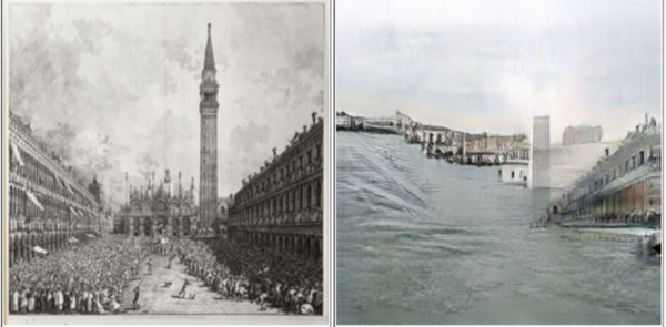
In the initial model results, we observed that the generator was learning to overwrite particular challenging aspects of images properly rather than modifying them coherently. This resulted in a worse performing model: some structures in the input such as boats or features in building were deleted, as we can see in Fig. 3. To combat this issue, we imagined and implemented an edge detection inverse loss component into the model.

We use the Canny edge detection algorithm. This algorithm allows us to convert the images into purely edges, by applying a succession of Gaussian filters and other components. Then, taking the edge images of the generator input and output, we used SSIM to compare their similarity. After multiplying the similarity score by our edge loss parameter value (which lets us control how much the model takes the edge loss into account) we subtract the score from the standard loss created by the discriminator. The forces the generator to learn not just to create images which satisfy the discriminator, but also which maintain the edges (and thus the structures and objects) from the original input image.

Spectral Normalization

Another modification we made to prevent the model from "over-learning" the target data and generating new structures in place of the input image structures was adding spectral norm to the resnet blocks. Spectral normalization has been documented to combat mode collapse very efficiently, and thus is relevant in this case as our problem it broadly analagous to mode collapse. Spectral normalization normalizes the weight for each layer with the spectral norm σ(W) such that the Lipschitz constant for each layer as well as the whole network equals one. With Spectral Normalization, we renormalize the weights whenever it is updated. This creates a network that mitigates gradient explosion problems and mode collapse.

Self-attention layers

Todo

Performance evaluation

Fig. 4: Low canny filters, over-representing the red hues of the image

Fig. 5: Cloud transformed into a building, due to the high learning rate/high relative number of learning epochs

One of the foremost challenges in the project was to select our performance evaluation criteria: since the goal is to render paintings and drawings photorealistic, we had to rely on our subjective judgement of what we consider to be photorealistic.

We chose to focus on the following criteria to evaluate the performances of our model:

• Appropriate coloration according to reality: correctly colored buildings, no over-saturation for a single color.
• Consistent structures: in the rendering, buildings are not removed, and the structures are not modified too much, mainly enhancing or reducing detail to make the image more realistic.
• Not overfitting to noise: sometimes paintings can hold a great amount of detail in brush strokes, for instance in clouds, and the GAN model tends to interpret some of these details as structure details, whereas such noise should be ignored most of the time.
• Comprehensible rendering of underwater Venice (only underwater model): we aim to show a portrayal of an underwater version of Venice that has a similar structure as in the input photo, with appropriate coloration and light reflection to make it look like it is indeed underwater.

Fig. 6: Input Photo of Venice (left) and output underwater version (right) of the final model

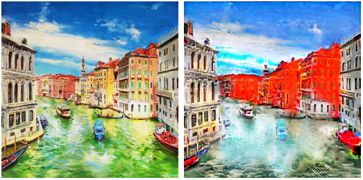
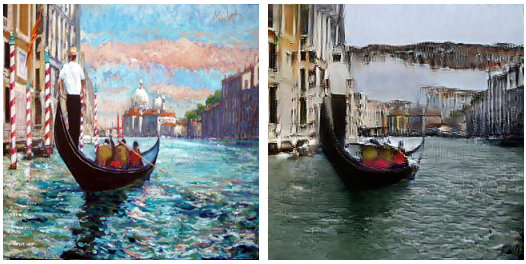
We can see in Fig. 4 and Fig. 5 how we observed bad performances in the models while tuning parameters, according to these evaluation criteria. In Fig. 4, we can see how the low Canny filter parameters caused the over-representation of the colour red from the input image in the output image. In Fig. 5, we see how the model overfits to the noise in the input image, transforming a cloud into a building.

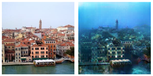
To obtain the final underwater model (Fig.6), we mainly focused on learning optimization and edge detection loss.

Estimated Relative Sea-Level Rise in Venice

In order to reliably depict the rising sea level in the coming decades, we have consulted relevant research literature.

To predict the sea-level rise in Venice, several variables have to be taken into account. The natural and anthropogenic land subsidence of Venice, the rising sea level due to climate change and the additional sinking due to increased groundwater extraction (excessively occurred between 1920 and 1970).

A measuring station of the local sea level in Venice wasn’t installed until 1897, so that the sea level of the previous centuries had to be estimated. It was determined with the help of the paintings by Veronese (i.e. 1571) and Canaletto (i.e. 1727–1758) and by measuring the submersion of the water stairs of the historic palaces along the Grand Canal.

In order to simplify the highly complex topic and its strong fluctuations, we opted for Roy Butterfield's linear fitting estimate of Venice’s Relative Sea-Level change of 1.43mm/year (without taking climate change into account) and put the worst-case RCP8.5 Sea-Level scenario of the IPCC on top of it.

Because our visualization of the rising sea level ignores even the angle of view and the horizon height of the input photos, we consider the increasing unscientific nature of the forecasts over the years, especially beyond 2100, to be irrelevant for our task. The core of this visualization is to envision the threat posed by the rising sea-level.

Quality Assessment

Model results

Photorealistic Venice (color and monochrome)

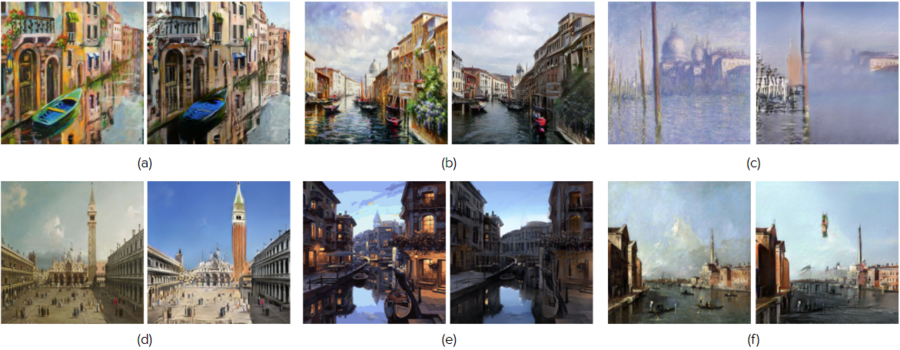
We present the results of the color and monochrome models in Fig. 7 and 8, respectively. The renderings of both models are quite impressive: each model is able to learn colors and structures quite well, although both models appear to have similar caveats in their learning.

The color model is able to effectively attenuate bright colors in Fig. 7a, 7b, 7e. It also enhances lackluster colors in Fig. 7d for the sky and it even renders St Mark's campanile wider and significantly brighter as it is in reality. In addition to correcting some of the structures to make them more realistic, it is able to attenuate some edges properly, for instance the clouds in Fig. 7b, 7d and 7e. However, if the clouds are particularly detailed in the color painting, the the model attempts to generate structures from them, as we see in Fig. 7f.

We can see that the color model performs generally well on more typical color palettes (enhanced compared to reality, as in Fig. 7a and 7b; muted compared to reality as in Fig. 7d). However, the model does not perform as well with more rare color palettes, as we see in Fig. 7c. This is because we had few images in the color painting dataset of similar colors, and thus the model has not been able to properly learn how to perform a style transfer from like colors.

The monochrome model TODO

Overall, both models are very effective at the first two performance evaluation goals: appropriate coloration and realistic rendering of the painting/drawing subjects. The colors in both photorealistic renderings are consistent with reality, and both models make an effort to generate more realistic structures, by learning patterns and details that are seen in reality and are often portrayed in drawings and paintings. In both models however, the models overfit for noise in the clouds in input art, by generating structures in the clouds. This is caused by the trade-off of using edge detection: the models are better at recognizing structures that do exist, but it can also sometimes generate structures where they do not actually exist.

Fig. 7: Color model sample results (left: input color painting, right: photorealistic rendering)

Fig. 8: Monochrome model sample results (left: input monochrome painting/drawing, right: photorealistic rendering)

Underwater Venice

TODO

Appropriate coloration according to reality

Consistent structures (realistic rendering of subjects)

Not overfitting to noise

Comprehensible rendering of underwater Venice

Fig. 9: Underwater model sample results (left: input photo, right: underwater rendering of photo)

Limitations

We acknowledge several limitations of our methods, mainly caused by incorrect assumptions and time constraints.

One incorrect assumption that was made in the start of the project was that we would be able to see differences in model performances using quantitative measures, such as generator loss. In the initial test of the edge detection component, we used sweeps to observe generator and NCE loss of different models, to choose how to select the optimal models. However, after initial tests, we observed that the quantitative loss metrics did not vary drastically between the various models, whereas the outputs were significantly different. We can see the loss functions of four trained models in Fig. 10, compared to each of their outputs for the same input image in Fig. 11. We thus continued to test models by manually evaluating their results, considering factors described in the previous section.

Another limitation to our project was that in addition to the many preexisting hyperparameters of the CUT model, we added multiple extensions, which made the number of parameters to test unreasonable in the time frame that we had. We tested as many hyperparameter configurations as we could in the time frame given, occasionally causing us to delay our planning, but if we had a larger time frame we could further optimize the model performance by testing more configurations with a larger number of training epochs.

Fig. 10: Loss metrics (visualized using WandB)

Fig. 11: Model outputs for the four models trained in Fig. 10 (cp1 to cp4 from left to right)

Further work

In a further work, one could test more combinations of hyperparameters for our models, in addition to using larger and more images for the training. One could also adapt to more art styles (impressionist paintings, more sketch-like drawings) for a better performance for the models for more unusual input drawings and paintings.

This model could also be used to create photorealistic renderings from paintings of other cities, such as Paris or Rome, although it would have to be retrained on images of these cities. We hope that our project will allow others to see historical portrayals of Venice in a more modern way, to better understand how Venice looked in its earlier days.

Links

• Github repository for this project
• GitHub: Contrastive Unpaired Translation
• Wikipedia: Canny edge detector (for edge loss implementation)
• Fondazione Giorgio Cini

References

- ↑ Taesung Park and Alexei A. Efros and Richard Zhang and Jun-Yan Zhu: Contrastive Learning for Unpaired Image-to-Image Translation, in: European Conference on Computer Vision, Berkely, 2020.